As already commented so far, for the linear wave equation to be satisfied in any number of dimensions the condition (here shown for three dimensions)
$$ k^{2} = k_{x}^{2} + k_{y}^{2} + k_{z}^{2}$$
must hold. Now, consider the complex exponential solution of the linearised wave equation of the form
$$ p(x, y, z, t) = A e^{-j \left( k_{x} x + k_{y} y + k_{z} z\right)} e^{-j \omega t}$$
The last term of above equation is the temporal term and will be skipped for the moment. The above solution represents a plane wave travelling in the direction specified by the first exponential term. To see that better consider the exponent (omitting the imaginary unit) to be of the equivalent form
$$ \mathbf{k_{x}} + \mathbf{k_{y}} + \mathbf{k_{z}} = k_{x} \mathbf{e}_{x} + k_{y} \mathbf{e}_{y} + k_{z} \mathbf{e}_{z}$$
where with bold are indicated vector values and $\mathbf{e}_{x}$, $\mathbf{e}_{y}$ and $\mathbf{e}_{z}$ represent unit vectors pointing along the specified directions. Thus, their weighted vector addition (weights being the $k$ values) forms a vector pointing towards a specific direction, albeit not a unit vector anymore. Nevertheless, the resultant vector points towards the direction of propagation of the plane wave in 3D. Of course, if any of the $k_{i}$ values is identically 0 then the propagation happens in only two dimensions, like in your case that happens in the $x-y$ plane.
Now, moving to your case specifically. In order to "create" the direction of your plane wave you have to create the components of the resultant unit vector pointing towards the direction of propagation. This is quite easy for the 2D case. In order to create a unit vector pointing towards a specific direction two specific conditions must be satisfied. First, the magnitude of the vector to be 1 and second, its angle with the $x$ axis must equal the angle of propagation. An easy choice that satisfies both conditions is
$$ \mathbf{e}_{2} = \left[ \cos \left( \theta \right), \sin \left( \theta \right) \right] $$
where the subscript denotes that this is vector in $\mathbb{R}^{2}$. So, the resulting equation (for two dimensions this time) becomes
$$ p(x, y, t) = A e^{-j \left( k_{x} \cos \left(\theta\right) x + k_{y} \sin \left(\theta\right) y \right)} e^{-j \omega t}$$
Now the good part. Observing the above equation you may notice that on each dimension (Cartesian direction) you end up with a (co)sinusoidal component. Of course their "amplitude" is $k_{i}$. Do not be tempted to consider this to be the actual amplitude of each component, it's just a scaling factor and the final quantity ($k_{i} \cos \left( \theta \right)$, or similarly $k_{i} \sin \left( \theta \right)$), which is a constant for specific temporal frequency (keep in mind that $k = \frac{\omega}{c} = \frac{2 \pi f}{c}$ with $c$ being the speed of sound and $f$ the temporal frequency) and direction (this is dictated by the result of $\cos \left( \theta \right)$ or $\sin \left( \theta \right)$ which depends only on the angle of propagation $\theta$), is just a scalar that declares the spatial frequency of the plane wave on each direction of propagation. A simple example of this would be a plane wave traveling parallel to the $x$ axis. The expression is
$$ p(x, y, t) = A e^{-j \left( k_{x} \cos \left(\theta\right) x + k_{y} \sin \left(\theta\right) y \right)} e^{-j \omega t} \implies p(x, y, t) = A e^{-j \left( k_{x} \cos \left(0 \right) x + k_{y} \sin \left(0 \right) y \right)} e^{-j \omega t} \implies p(x, y, t) = A e^{-j k_{x} x} e^{-j \omega t} $$
Please note that we are still in two dimensions. If you get the real part you end up with the well known (co)sinusoidal solution
$$ p(x, y, t) = A \cos \left( \omega t - k_{x} x \right) $$
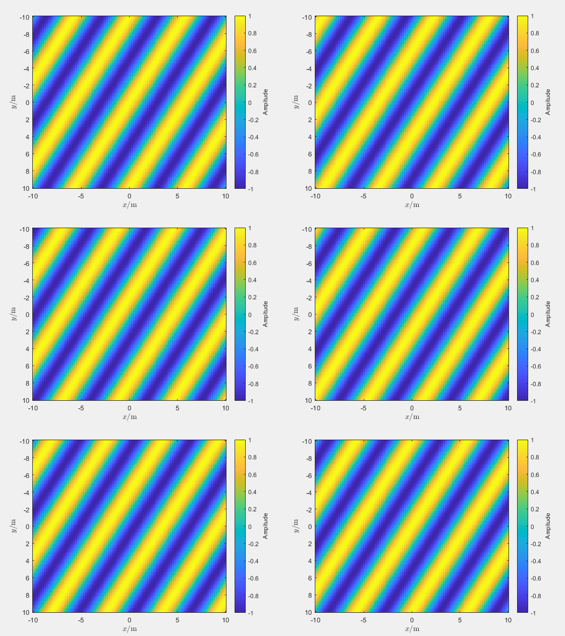
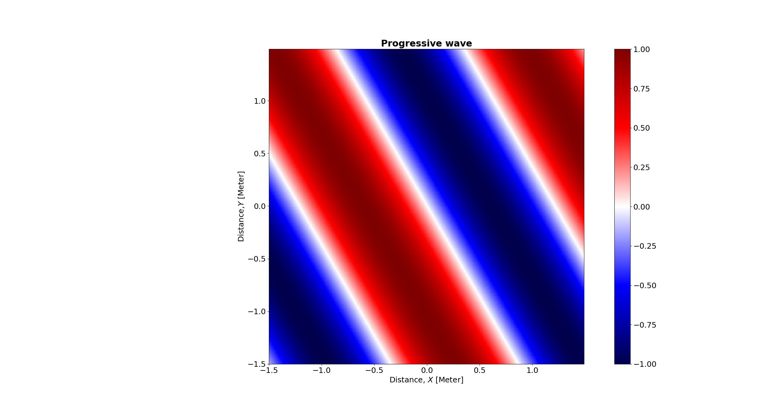
Below you can see an illustration of such a wave.

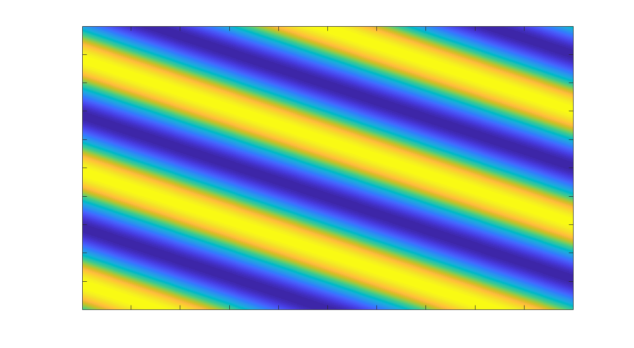
The picture shows a monochromatic plane wave with temporal frequency equal to $100 Hz$. Similarly, if you use a different $\theta$ and plug it in the general equation you end up with a plane wave traveling in the direction dictated by the $\theta$ parameter. An example of a monochromatic wave with the same temporal frequency and direction of travel $60^{o}$ is shown in the next image.

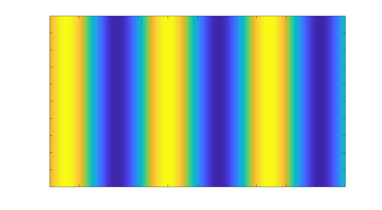
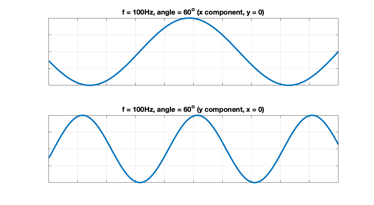
If you take a closer look, especially easy to notice on the boundaries of the screen, you may see that on each direction ($x$ and $y$ axes) there are (co)sinusoidal components forming. Those are depicted below for the plane wave of the last (second) picture (please note that the origin of the system lies in the top left corner. This is due to MATLAB's plotting function used. I apologise for the inconvenience)

Now, I believe it is quite clear that those two components constitute the spatial components of the plane wave. These are also utilised in the so called "Plane wave decomposition" methods if further simplification of the plane waves is needed. They become useful in 3D audio and array processing techniques. The frequency of the spatial components is the spatial frequency of each component governed by (actually being identical to) the respective wavenumbers ($k_{x}$ and $k_{y}$ in this case).
At this point, it is instructive to say (and easy to notice) that if you offset the constant directions by a value, the spatial component will experience a phase shift. For example, if the spatial components were not plotted for $y = 0$ and $x = 0$ but for some arbitrary $x$ and $y$ values, the corresponding spatial components would experience a phase shift. You can have a look at the respective spatial components by inspecting the 2D plot of the wave in the middle of the figure.
Although we have covered a lot of the road we haven't touched upon the temporal dimension yet. What you've seen show far is a snapshot of the monochromatic plane waves we have been talking about. Of course, if you were to take many such snapshots at different time instances you could create a "movie" of the propagating wave. The problem is that you cannot tell which way the wave is progressing towards. This is due to the fact that deal with the steady state and we cannot deduce any such information from what we have at hand. It's like floating in the middle of the ocean and moving up and down due to waves but with absolutely no mass transfer from the waves (this is essentially what linearised acoustic waves are). How would you be able to say which direction the waves are moving towards since you only know when you are at the peak and when you reach the lowest possible height? Well, the answer is you can't.
As for the velocity, it cannot be deduced from a temporal snapshot because time is "frozen". You look at the wave at a specific moment in time but in order to calculate speed you need at least two time instances to calculate the difference in position and divide by the duration ($c = \frac{x}{t}$). If you are allowed to let time change then you could possibly look for the duration between two maxima or minima (or whichever part of the cycle) and estimate the speed from that.
Code
The code to create the plots I presented can be seen below
%% Set parameters
c = 343; % Speed of sound
ang = 60; % Angle of propagation
f = [100]; % Temporal frequency
Lx = 10; % length of x dimension of the domain
Ly = 10; % length of y dimension of the domain
res = 1e-2; % Resolution of the lengths

% Calculate Variables
Lx = 0:res:Lx - res; % Calculate the x-axis
Ly = Ly - res:-res:0; % Calculate the y-axis
w = 2 * pi * f; % Radial frequency
k = w/c; % Wavenumber
kx = k .* sin(deg2rad(ang)); % x component of wavenumber
ky = k .* cos(deg2rad(ang)); % y component of wavenumber

%% Calculate signal
sig = zeros(2, length(Lx), length(Ly)); % Pre-allocate for speed

% Go through the positions (this is quite slow but is a straight forward implementation)
for xx = 1:length(Lx) % x dimension
    for yy = 1:length(Ly) % y dimension
        sig(1, xx, yy) = sin(w(1) - kx(1) * Lx(xx) - ky(1) * Ly(yy)); % Calculate the value of the plane wave on each position
    end
end

%% Visualise
figure("Name", "Plane Wave")
imagesc(squeeze(sig(1, :, :)));
xticklabels([])
yticklabels([])

figure("Name", "Components")
subplot(2, 1, 1)
temp = squeeze(sig(1, :, :));
plot(temp(1, :), 'LineWidth', 5);
grid on
xticklabels([])
yticklabels([])
title("f = " + num2str(f) + "Hz, angle = " + num2str(ang) + "^o (x component, y = 0)", 'FontSize', 24)

subplot(2, 1, 2)
plot(temp(:, 1), 'LineWidth', 5);
grid on
xticklabels([])
yticklabels([])
title("f = " + num2str(1) + "Hz, angle = " + num2str(ang) + "^o (y component, x = 0)", 'FontSize', 24)


