I currently work in the design of atomic clocks and precision frequency sources and pleased to report that the Allan Variance is still quite relevant and useful. In fact it's utility extends to convenient characterization of many non-stationary processes, well beyond its primary tool as a frequency stability assessment. (And as mentioned in its comments, it’s use to assess stability of accelerometers).
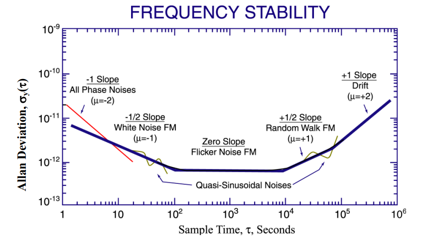
Traditional statistical approaches using the first and second order moments (mean and standard deviation, or equivalently squared as the variance) cannot be computed for non-stationary processes, since the variance will increase the longer you compute the parameter on the data set (diverging). The Allan Variance or Two-Sample Variance is a convenient statistical tool to provide a metric similar to the variance for non-stationary processes. It basically converts non-stationary data to stationary for a consistent metric that can be used to compare competing products or solutions. Applicable to other processes, I personally like how I can use the Allan Variance to quickly assess an optimum averaging time (what we would call the "Flicker Floor" if the independent variable is frequency), for which if we average up to that time we can get an improved estimate of the mean, but if we average any longer, the noise of that estimate only degrades. For example, this can then be applied to optimum time durations for channel equalization and estimation, or any process where we are computing a longer term average to estimate a parameter.
The following graphic copied from a NIST presentation shows how ADEV can reveal the different noise processes within a signal, and where there effects would be of concern (in terms of observation times, $\tau$). This was from a 2015 presentation by Marc Weiss and Kishan Shenoi.

I have further detailed the Allan Variance and its practical purpose at these other links starting with the link copied below (that includes links to other related posts):
Allan Variance vs Autocorrelation - Advantages

