4
$\begingroup$

Following up on a previous question, I wanted to understand how to solve an image deblurring problem using Variational methods in matlab or julia.

Given some original blurry image $f$, I would like to find the deblurred version $u$. $K$ is a function that essentially softens the edges of the image and takes $K: u \rightarrow f$. The statement of the problem involves minimizing the energy of the squared loss with an additional

$$ E(u)=\int_{\Omega}|D u|^{2} d x+\lambda \int_{\Omega}(K u-f)^{2} d x $$

I am taking the statement of the problem from the Vese and Guyader 2016 book.

Using the ADMM optimizer, the method can take a blurry image such as: Blurry Image

and recover a sharper image as below.

Sharpened Image

UPDATE:

The ADMM optimizer is often used to minimize these function, as are other similar methods like the split Bregman iteration. These splitting methods seem to break the objective function into separate parts and then interactively optimize each piece. I just wanted to understand how to set up that optimization with this particular deblurring problem, in particular setting up the regularization term $|Du|^2$. In the denoising problem the regularization was $|Du|$, so the answer to this question will provide and additional example of setting up ADMM. In particular the $|Du|^2$ should be convex whereas the $|Du|$ was not--since there might have been some special handling in the setup and execution of the optimizers in the denoising case that is not required in the deblurring case.

$\endgroup$
4
  • 1
    $\begingroup$ It seems you forgot to ask a question. "Please someone explain (complex topic)" isn't a great question in terms of scope. Please explain exactly what you've researched so far, and where you're stuck! To me, it seems you've gotten a very solid answer to your other question that addresses exactly this question, but I don't want to suggest this is a pure duplicate before I understand how you've progressed since you've read Royi's answer to your previous question! $\endgroup$ Commented Jun 2, 2021 at 15:23
  • $\begingroup$ @MarcusMüller thanks for your kind note. Yes my main motivation was to understand the coding of these models in term of the optimization algorithm. In my previous question, at the bottom of Royi's answer, he indicated that he had some additional code for deblurring and that I should post a new question about that. Hence, I was following up on that suggestion. In particular I would like to understand how to setup the additional regularization term in the ADMM optimizer--the $|Du|^2$ term, since it differs from the TV norm in the previous question. $\endgroup$
    – krishnab
    Commented Jun 2, 2021 at 22:12
  • $\begingroup$ But I can totally update the OP and specify that I want to focus on that regularization term. These ADMM or similar optimization routines seem to split the objective function into pieces and optimize those pieces in turn. Hence I just wanted to see another example so I can make sure I understand that splitting. $\endgroup$
    – krishnab
    Commented Jun 2, 2021 at 22:16
  • 1
    $\begingroup$ I mean, if you incorporate all the info you're giving in the comments here into this question, and it seems that's your intention, that makes for a very interesting question! $\endgroup$ Commented Jun 3, 2021 at 9:54

1 Answer 1

1
$\begingroup$

Remark: This is adapted from How to Solve Image Deblurring with Total Variation Prior Using ADMM?

Formulation of the Problem

I am solving the problem under the following assumptions:

  • The blurring operator is Linear and Spatially Invariant (Hence applied by convolution).
  • The blurring operator is known.
  • There is a measurement noise.

So the model is:

$$ \boldsymbol{y} = H \boldsymbol{x} + \boldsymbol{n} $$

Where $ H $ is the matrix form of the blurring kernel, $ \boldsymbol{n} $ is AWGN noise and $ \boldsymbol{x} $ is the reference image to be estimated.
In the model, we assume that $ D \boldsymbol{x} \sim \text{Exponential} \left( \lambda \right) $ (See Exponential Distribution).

Hence the optimization problem (Equivalent of the MAP Estimator) is given by:

$$ \arg \min_{\boldsymbol{x}} \frac{1}{2} {\left\| H \boldsymbol{x} - \boldsymbol{y} \right\|}_{2}^{2} + \lambda \operatorname{TV} \left( \boldsymbol{x} \right) = \arg \min_{x} \frac{1}{2} {\left\| H \boldsymbol{x} - \boldsymbol{y} \right\|}_{2}^{2} + \lambda {\left\| D \boldsymbol{x} \right\|}_{1} $$

Pay attention that this model makes sense only when noise is added as otherwise the TV term only smoothens the output. So the regularization of the TV allows to control between inversing the blurring operator and smoothing the noise.

Solution by ADMM

The ADMM problem will be formulated as:

$$ $$

$$\begin{aligned} \arg \min_{\boldsymbol{x}, \boldsymbol{z}} \quad & \frac{1}{2} {\left\| H \boldsymbol{x} - \boldsymbol{y} \right\|}_{2}^{2} + \lambda {\left\| \boldsymbol{z} \right\|}_{1} \\ \text{subject to} \quad & D \boldsymbol{x} = \boldsymbol{z} \end{aligned}$$

The ADMM will have 3 steps:

  1. vX = mC \ (vY + (paramRho * mD.' * (vZ - vU)));.
  2. vZ = ProxL1(mD * vX + vU, paramLambda / paramRho);.
  3. vU = vU + mD * vX - vZ;.

Where mC = decomposition(mH.' * mH + paramRho * (mD.' * mD), 'chol'); (That's the difference from How to Solve Image Denoising with Total Variation Prior Using ADMM?).
The parameter paramRho is the parameter of the ADMM solver.

I coded this solution in a MATLAB function - SolveLsTvAdmm().
I compared it to a reference by CVX:
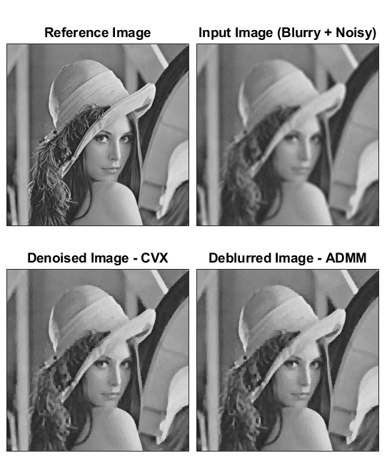
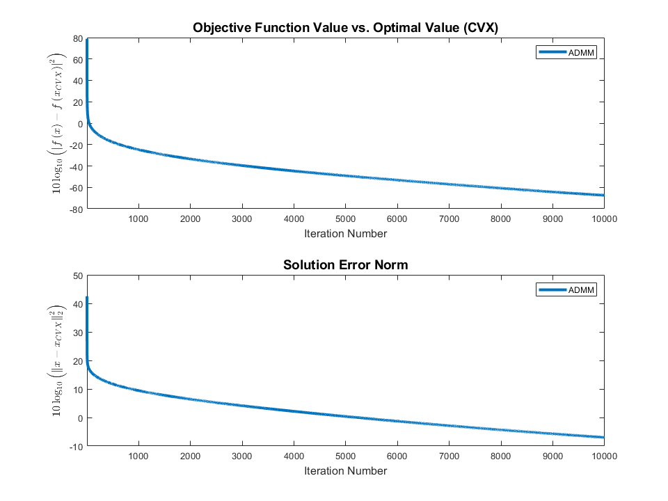
enter image description here enter image description here

In the above the noise level was 3 / 255 (Image was scaled to the range [0, 1]) and the blurring operator was Box Blur with radius of 2.
I didn't optimize the paramLambda to its optimal value. So one could get better results. Pay attention that for this low level of paramLambda and small size of an image the ADMM solver is slower then the direct solver of CVX.

The full code is available on my StackExchange Signal Processing Q75471 GitHub Repository (Look at the SignalProcessing\Q75471 folder).

The TV Term

In the code above I used the Anisotropic version of the Total Variation model (You may see What Does the Total Variation Norm Mean in the Context of Image Processing and The Meaning of the Terms Isotropic and Anisotropic in the Total Variation Framework).
If you're specifically after the Isotropic variation of the TV Norm then you'll have to replace the Prox Operator in my code and the derivation of the gradient.
Some resources on doing just that:

$\endgroup$
1

Your Answer

By clicking “Post Your Answer”, you agree to our terms of service and acknowledge you have read our privacy policy.

Not the answer you're looking for? Browse other questions tagged or ask your own question.