Negative instantaneous frequency with hilbert transform using scipy hilbert

Question

When I produce a chirp signal with a duration of 2 sec, sampling frequency of 200Hz, with frequencies ranging from 20Hz-100Hz, I get negative instantaneous frequencies using the scipy(Python) Hilbert transform. Here is my signal code:

    self.duration = 2
    self.fs = 200.0
    samples = int(self.fs * self.duration)
    self.time = np.arange(samples) / self.fs
    carrier = chirp(self.time, 20, self.time[-1], 100) 
    self.signal = carrier * (
        1 + 0.5 * np.cos(10 * 2.0 * np.pi * self.time)
    ) 

Here is my Hilbert transform code:

demean = data - np.mean(data)
hil = hilbert(demean)
inst_amplitude = np.abs(hil)
inst_phase = np.unwrap(np.angle(hil))
inst_frequency = np.diff(inst_phase) / (2 * np.pi) * sampling_frequency
inst_frequency = np.insert(inst_frequency, 0, 0)
regen_carrier = np.cos(inst_phase)

Here is the plot of the Hilbert properties:

Why are there negative instantaneous frequencies? I have been Googling the issue with zero luck finding an answer. Any input would be greatly appreciated.

UPDATE: I applied the exact same Hilbert transform code as above to a "real life" dataset with a sampling frequency of 800Hz. I am getting negative instantaneous frequencies in the middle of the data, not just at the edges. I don't think I am allowed to show the data as it is proprietary, so sorry on that front. Any insight as to why I am seeing negative frequencies in the middle of my data and not just at the edges?

UPDATE #2 I went ahead and generated a synthetic chirp signal with multiple frequency sweeps using scipy.signal.sweep_poly and I am getting negative instantaneous frequencies in the middle of my data.

Here is the code for my new signal (duration of 50sec and sampling frequency of 100):

    self.duration = 50
    self.fs = 100.0
    samples = int(self.fs * self.duration)
    self.time = np.arange(samples) / self.fs
    p = np.poly1d([0.025, -0.36, 1.25, 2.0])
    self.signal = sweep_poly(self.time, p) 
    

Here is the plot of the new signal's Hilbert properties:

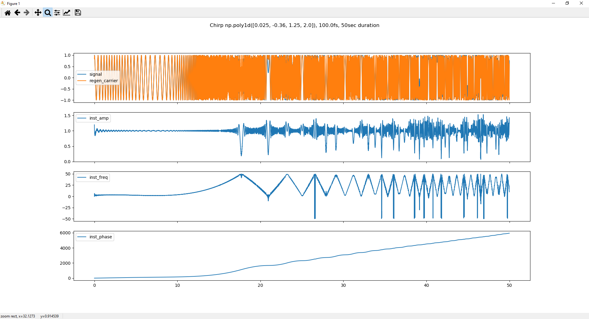
Here's the same image, but zoomed in where there are negative instantaneous frequencies in the middle of my data:

Why are there negative instantaneous frequencies in the middle of my data? There are definitely no edges in the middle of my data, so it's not an edge effect.

UPDATE #3 I added random noise to the exact same signal using the following code:

    self.duration = 50
    self.fs = 100.0
    samples = int(self.fs * self.duration)
    self.time = np.arange(samples) / self.fs
    p = np.poly1d([0.025, -0.36, 1.25, 2.0])
    carrier = sweep_poly(self.time, p)  # Carrier signal
    noise = np.random.normal(0, 1, carrier.shape)
    self.signal = carrier + noise

Here is the plot of the noisy Hilbert transform properties:

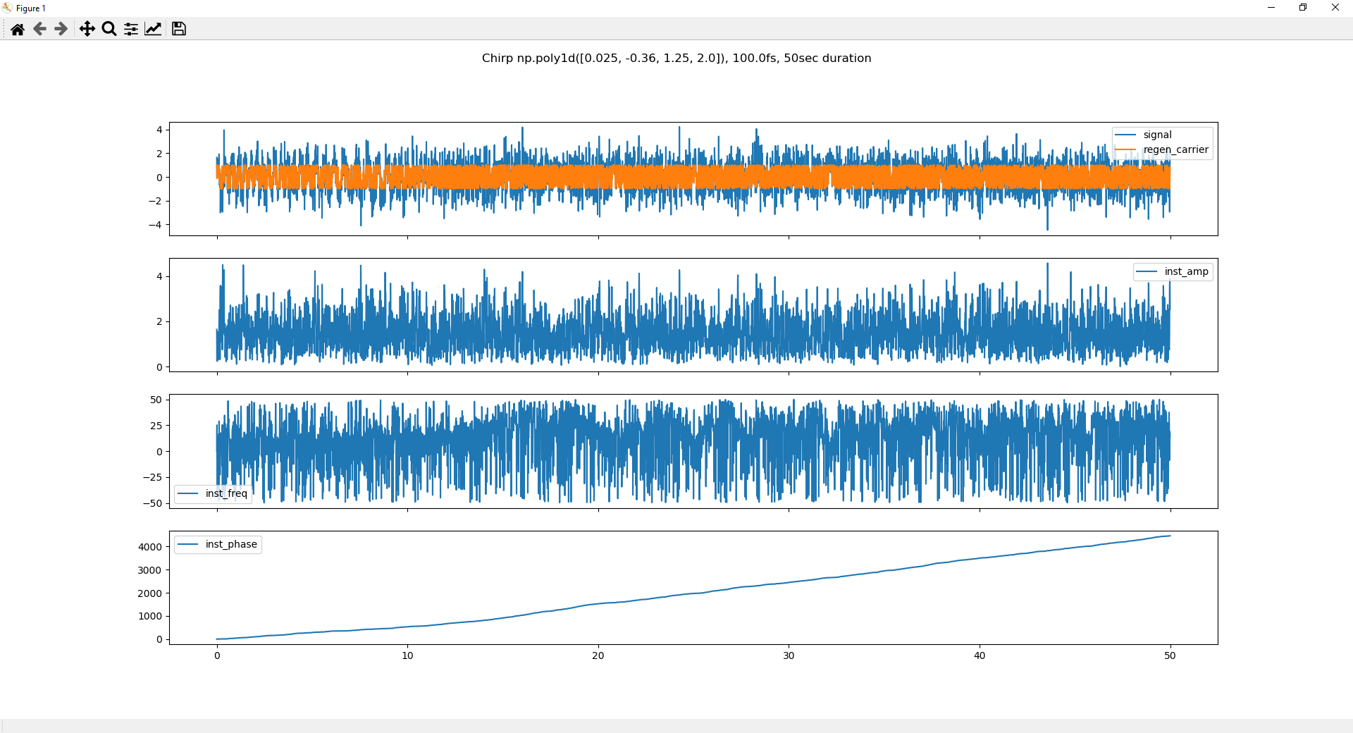
Even more negative frequencies! Why is this happening?

UPDATE #4 I decided to multiply 2 sine functions with two different constant frequencies together to see what I get. There is no noise in this instance. Here is my code:

    self.duration = 2
    self.fs = 100
    samples = int(self.fs * self.duration)
    self.time = np.arange(samples) / self.fs
    self.signal1 = np.sin(1 * 2.0 * np.pi * self.time)
    self.signal2 = np.sin(9 * 2.0 * np.pi * self.time)
    self.signal = self.signal1 * self.signal2

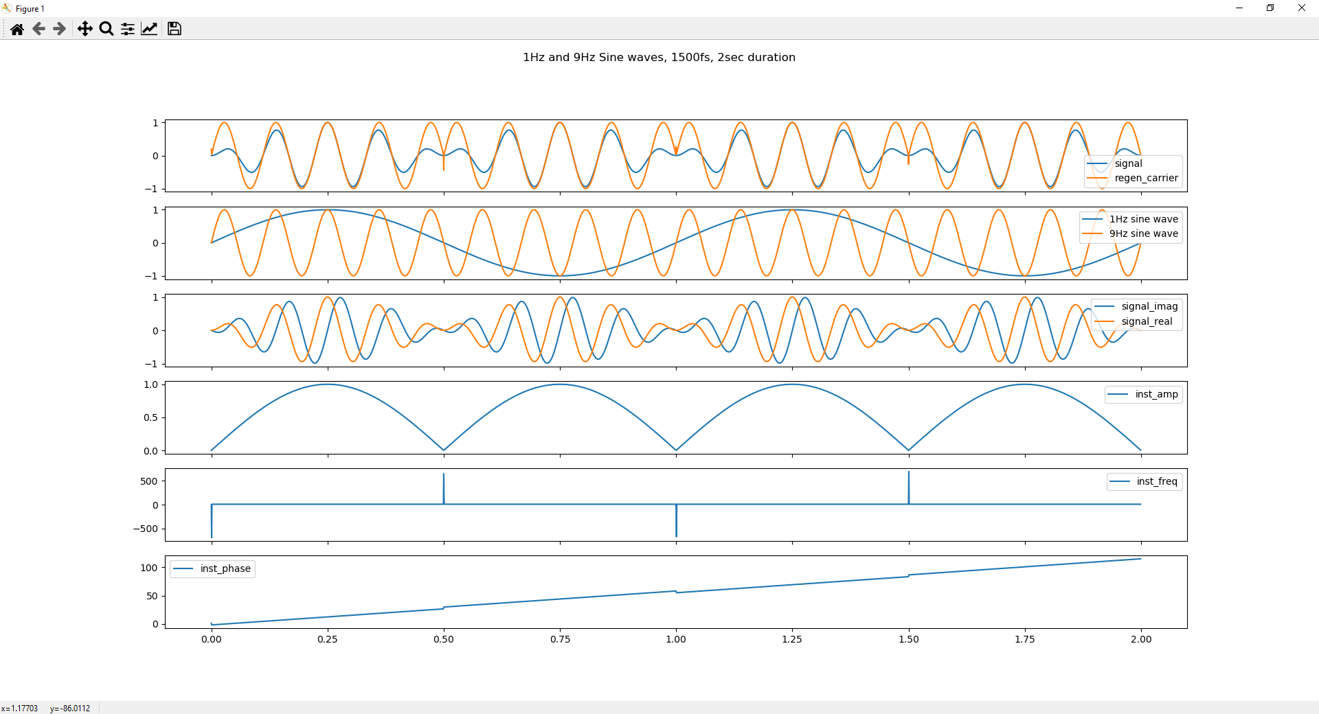
Here is the plot of the resulting Hilbert properties:

If I change the sampling frequency, the magnitude and sign of the instantaneous frequency spikes change! Here are a few examples (the sampling frequency used is in the title of the image):

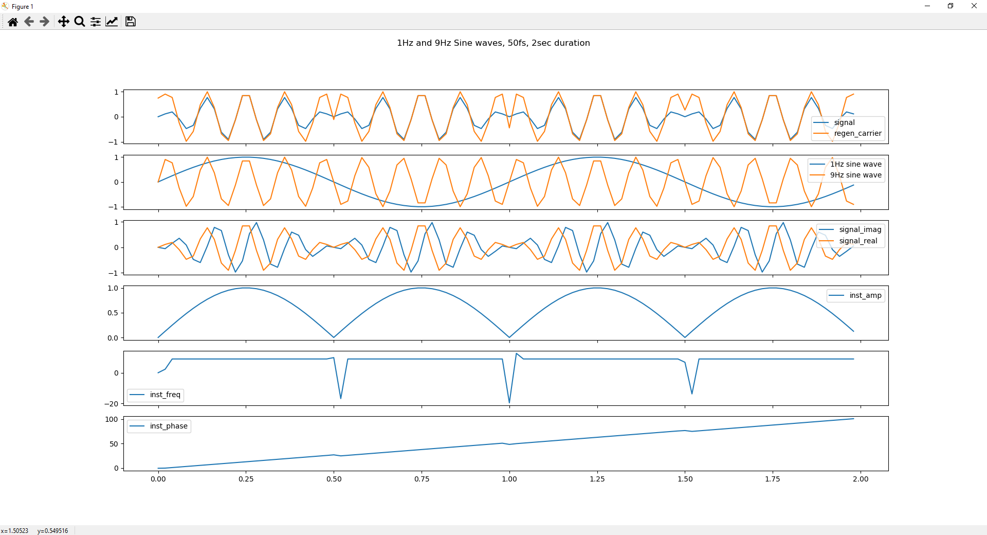
Something about the phase calculation is unstable and the sampling frequency seems to alter things. No I am even more curious as to what is happening.

Thanks!

Answer 1

It looks like artifacts due to the derivative. I used this code in Octave:

fs=300;
t=[0:1/fs:2];
c=chirp(t, 20, 2, 100);
s=c.*(1+0.5*cos(2*pi*10*t));
h=hilbert(s);
m=abs(h);
a=diff(unwrap(arg(h)))/2/pi*fs;
plot(m,"",a)

and this is what comes out:

I also tested the equivalent of this in LTspice and, without any form of unwrapping, this is the result:

where V(mag) is the result of hypot() (m), V(signal) is s, V(freq) is the frequency for the FM, and V(demod) is a. All are delayed (for matching I/O) by 23/2/200 which represents the order of the Hilbert transformer (Hamming window), divided by two (group delay) and by the sampling frequency (200).

My guess: don't take for granted the result of the differentiator and try to take a finer comb to it (is this a pun? not intended).