How to model transfer functions using Python (without using higher level packages) and plot the magnitude and phase response?

Question

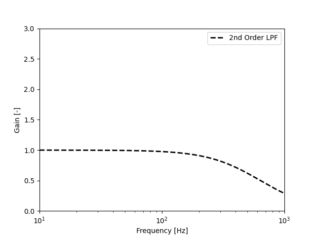
I'm trying to model a transfer function in Python and thought I could do it by simply plotting the transfer function at many frequencies. This seemed to work for a 2nd order LPF. See the below figure.

A bit of sample code would be like:

s = np.arange(10 * 2 * np.pi, 1000 * 2 * np.pi, 10) # Creates vector of frequencies in rad/s
lpf = np.zeros(len(s))  # Initializes lowpass filter vector

for k in range(len(s)):
   lpf[k] = lpfilt_func(s[k])  # Calls LPF function with TF = cutoff_freq ** 2 / (s + cutoff_freq) ** 2

To get the frequency response, instead of using s as a real number, I changed s to a complex number using the built-in function complex(0, s) and calculated the magnitude and phase as follows:

for k in range(len(s)):
   lpf[k] = lpfilt_func(complex(0, s[k]))
   gain_lpf[k] = np.absolute(lpfilt_func(complex(0, s[k])))
   phase_lpf[k] = np.angle(lpfilt_func(complex(0, s[k]))) * 180 / np.pi  # Phase in deg

I think this is essentially like setting $s = j\omega$ and then calculating the magnitude as $|LPF| = \sqrt{A^2 + B^2}$ and the phase response as $\angle{LPF} = \angle{(B/A)}$.

Is this a valid method to calculate the frequency response of a transfer function? Is this conversion of s from a real number to a complex number valid?

Answer 1

If the response is real you need not convert it to complex in order to compute the magnitude, but the process is correct for complex and real number since the abs function will use complex conjugate product prior to taking the square root. If it was real, there would be a trivial phase response since the phase would always be 0 degrees. This would not be a causal system so not a realistic example to have a real frequency response. For complex cases the approach used is correct for magnitude and phase, just not the most efficient.

To confirm results (or to compute directly), use the freqs and freqz commands that are part of scipy.signal for continuous-domain (s) and discrete-domain (z) transfer functions.

For example the transfer function

$$H(s) = \frac{s+1}{s+4s+4}$$ could be plotted using:

w,h = scipy.signal.freqs([1, 1], [1, 4, 4])

Returning the frequency (w) and complex response (h)

Read the help for both of those functions (also available under same name in MATLAB and Octave) for further info.

For MIMO systems the control package has this all worked out as part of the bode function.