Inverse Hilbert Transform

Question

The Hilbert Transform of a 1D/real-valued vector signal returns the analytic signal, x, from a real data sequence, xr. The analytic signal x = xr + jxi has a real part, xr, which is the original data, and an imaginary part, xi, which contains the Hilbert transform.

hilbert uses a four-step algorithm:

1. Calculate the FFT of the input sequence, storing the result in a vector x.

2. Create a vector h whose elements h(i) have the values:

     1 for i = 1, (n/2)+1

     2 for i = 2, 3, ... , (n/2)

     0 for i = (n/2)+2, ... , n

3. Calculate the element-wise product of x and h.

4. Calculate the inverse FFT of the sequence obtained in step 3 and returns the first n elements of the result.

This algorithm was first introduced in [8]. A python implementation of this can be seen bellow:

from scipy import linalg, fft as sp_fft
import numpy as np

def hilbert(x, N=None, axis=-1):
       
        x = np.asarray(x)
        if np.iscomplexobj(x):
            raise ValueError("x must be real.")
        if N is None:
            N = x.shape[axis]
        if N <= 0:
            raise ValueError("N must be positive.")
        print(x.shape,N,axis)
    
        Xf = sp_fft.fft(x, N, axis=axis)
        print(Xf.shape)
        #plt.plot(Xf)
        #plt.show()
        h = np.zeros(N)
        #plt.plot(h)
        #plt.show()
        if N % 2 == 0:
            h[0] = h[N // 2] = 1
            h[1:N // 2] = 2
        else:
            h[0] = 1
            h[1:(N + 1) // 2] = 2
        print(h)
    
        if x.ndim > 1:
            ind = [np.newaxis] * x.ndim
            ind[axis] = slice(None)
            h = h[tuple(ind)]
        x = sp_fft.ifft(Xf * h, axis=axis)
        return x 

This code was taken form Scipy implementation Scipy.signal.hilbert. I am looking to invert/reverse this process (inverse_hilbert), the best description i have found to do this is from Mathworks Inverse Hilbert Transform

However the real and complex arrays currently have me at a loss not sure how this feeds into this equation, or if this is the correct equation as wikipedia has a different equation to my understanding.

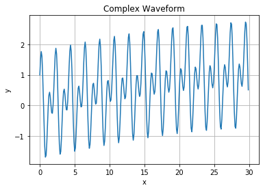
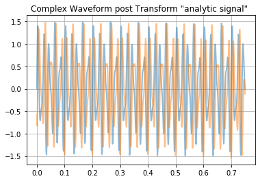
If we create a random complex signal and compute the hilbert Transform on it we get the following 2 arrays one real and one imagery. I am looking to reverse this transform any help would be appreciated.

import matplotlib.pyplot as plt

x = np.arange(0, 30, 0.1);
y = np.sin(0.05*x)+np.sin(6*x)+np.cos(3*x)  
plt.plot(x,y)
plt.title('Complex Waveform')
plt.xlabel('x')
plt.ylabel('y')
plt.grid()
plt.show()

x_a = hilbert(y)

plt.plot(x,x_a.real, label='Hilbert Real', alpha=0.5, lw=2)
plt.plot(x,x_a.imag, label='Hilbert Imag', alpha=0.5, lw=2)
plt.grid()

Any comments here to help my under standing would be appreciated, really looking for a step by step way to reverse this transformation.

[8]: Marple, S. L. “Computing the Discrete-Time Analytic Signal via FFT.” IEEE® Transactions on Signal Processing. Vol. 47, 1999, pp. 2600–2603.

Answer 1

I think the confusion comes from the fact that the command hilbert in Scipy (and also in Matlab/Octave) does not just compute the Hilbert transform, but its output is the analytic signal. So if $x(t)$ is the (real-valued) input to such a function, its (complex-valued) output is

$$y(t)=x(t)+j\mathcal{H}\{x(t)\}\tag{1}$$

Clearly, if you want to obtain $x(t)$ from $y(t)$, you just need to take its real part.

Concerning the inverse Hilbert transform, as you've already found out, the following holds:

$$\mathcal{H}^{-1}\{x(t)\}=-\mathcal{H}\{x(t)\}\tag{2}$$

The relation $(2)$ holds no matter if $x(t)$ is real-valued or complex-valued. However, if you use the function hilbert on a complex-valued signal, you throw away information that cannot be retrieved, because you throw away the negative frequencies, which are not redundant for complex-valued signals (unlike for real-valued signals). So the function hilbert cannot be inverted if the signal is complex-valued.

Answer 2

The Hilbert transform in (scipy.signal.hilbert) performs the following operations:

1. Making the data complex (by setting 0 as the phase value of each sample)
2. Computes the FFT
3. Zeros the negative frequencies
4. Scale the data by a factor of 2
5. Computes the iFFT

(see https://docs.scipy.org/doc/scipy/reference/generated/scipy.signal.hilbert.html)

note: The scipy.signal.hilbert function doubles the information, with the real to complex conversion. Since the number of samples stays the same, while the complex samples contains double the information. Alternatively the negative frequencies can be removed, instead of zeroing it. (For more info on the r2c FFT see https://github.com/HEnquist/realfft.)

To compute the inverse of the Hilbert transform (scipy.signal.hilbert) you can simply perform the reverse.

1. Compute the FFT
2. Remove the negative frequencies (redundant information)
3. Scale by a factor of 0.5
4. Compute the iFFT

The following code worked for me to calculate the inverse of the scipy.signal.hilbert function:

def invHilbert(cData):
   cFreqData = scipy.fft.fft(data)[:(len(cData//2+1)]
   data = 0.5*scipy.fft.irfft(cFreqData)
   return data

note: The code is for even number of samples, you might need to alter "[:(len(cData//2+1)]" to make it work for uneven number of samples.

note: The irfft performs a complex to real value iFFT.

The following is the result of a chirp signal, before and after Hilbert and invHilbert functions. (Fs = 48000, BW = 5000, number of samples = 100)

The following is the result of a chirp signal, before and after Hilbert and invHilbert functions. (Fs = 48000, BW = 500, number of samples = 10000)