7
$\begingroup$

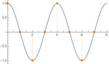
I'm experimenting with the Inverse Discrete Fourier Transform. Starting from the two-cycles continuous $x(t)$ signal below:

enter image description here

I have the discrete signal $x(n) = \{ 1, 0, -1, 0, 1, 0, -1, 0 \}$ leading to the 8 points DFT $X_0(n) = \{ 0, 0, 4, 0, 0, 0, 4, 0 \}$

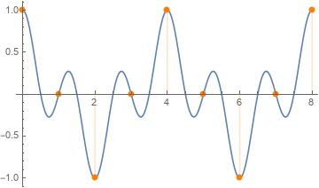
Now, if I use the IDFT on $X_0$, I obtain $x_0$ looking like that (the blue curve is the real part of the IDFT $Re[x_0(t)]$):

enter image description here

Here $x_0(n) = x(n)$ for integer values ($n = 0, 1, 2, \dots 7$). I understand I do not get back the continuous $x(t)$ function because of aliasing. I would explain that by saying on $x_0(t)$, there is a second signal, above the Nyquist frequency, and "riding" the "carrier"1

I read about zero padding, so I tried to add $k$ extra zeros in the middle of $X_0(t)$ and now, if I perform the IDFT, I obtain the following results:

1. With 8 extra values

I have $X_{k=8}(t) = \{ 0, 0, 4, 0, \underbrace{\mathbf{0, 0, 0, 0, 0, 0, 0, 0}}_\text{8 extra bins}, 0, 0, 4, 0 \}$, leading to $x_{k=8}(t)$: enter image description here
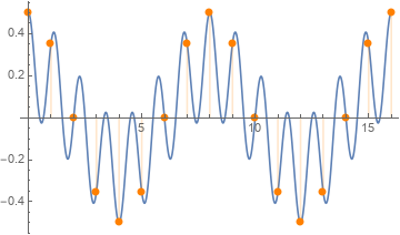
2. With 24 extra values

I have $X_{k=24}(t) = \{ 0, 0, 4, 0, \underbrace{\mathbf{0, 0, 0, 0, \dots, 0, 0, 0}}_\text{24 extra bins}, 0, 0, 4, 0 \}$, leading to $x_{k=24}(t)$: enter image description here
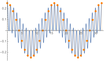
3. The problem

Adding more bins proportionally decreased the amplitude of the rebuild signal and increase the frequency of the signal riding the carrier. I think I understand both phenomenons.

However, I can't find an intuitive way of explaining why, at integer positions (the orange dots), $x_k(n)$ reproduces more and more accurately the original shape of the $x(t)$ signal.


1Do not hesitate to edit the question if I don't use the correct vocabulary here.

$\endgroup$
4
  • 2
    $\begingroup$ Hi. What is that blue curve in your 2nd plot? How did you compute that curve's values so that you could plot it? Your original x(n) sequence is two cycles of a cosine sequence whose frequency is Fs/2 Hz. Why do you think your original x(n) sequence contained multiple sinusoidal signals. $\endgroup$ Commented Dec 17, 2019 at 3:16
  • $\begingroup$ Thanks for the comment @Richard. I failed to mention it in the question but this is strongly inspired from exercise 3.21 in your book "Understanding Digital Signal Processing". The blue curve is the real part of the IDFT. Here is how I understand it: (1) the original sequence $x(n)$ is two cycles of a cosine. (2) Since this is a real signal, that leads to a DFT where $X(0, \dots , N/2-1) = X(N/2, \dots , N-1)$ So each bin is replicated at $n+N/2$. (3) When I build a new $x_0$ signal from that, it's made not of one, but two cosines. The original one and its replica. Or am I wrong? $\endgroup$ Commented Dec 17, 2019 at 11:09
  • 2
    $\begingroup$ Hi Sylvain. Send me a private e-mail to: [email protected] and I will send you the Solution to my Homework Problem 3.21. After reading my Solution 3.21, if you have any additional questions you can send them to me. $\endgroup$ Commented Dec 17, 2019 at 11:48
  • $\begingroup$ @SylvainLeroux, I think a full derivation is given at dsp.stackexchange.com/questions/72433. $\endgroup$
    – Mark
    Commented Nov 29, 2021 at 9:11

2 Answers 2

6
$\begingroup$

What you are experiencing is technically called interpolation by DFT; i.e., interpolating a time-domain sequence $x[n]$ by properly zero filling the middle portion of it's DFT $X[k]$ (and taking the inverse DFT to get the time domain interpolated sequence).

Typically, interpolation is described and performed in the time-domain, but equivalently possible in the frequency-domain, as a consequence of Fourier theorems.

Interpolation described in the time-domain:

$$ x[n] \rightarrow ({\uparrow L}) \rightarrow w[n] \rightarrow \boxed{LPF} \rightarrow y[n]$$

Input sequence $x[n]$ is of length $N$, expanded sequence $w[n]$ is of length $M = N \times L$, and the LPF has a Gain = L and discrete-time cutoff frequency of $\omega_c = \pi/L$ radians per sample.

The relation in the frequency-domain is such that if $X[k]$ is the N-point DFT of $x[n]$, then $W[k] = X[k]$ is the $M = L \times N$ point DFT of the sequence $w[n]$. Inded, $W[k]$ is an L-fold copy of $X[k]$. Let the DFT of the LPF be $H[k]$, which is also $M = L \times N$ points.

$$ H[k] = \begin{cases}{ L ~~~,~~~-N/2 \leq k \leq N/2 \\ 0 ~~~~, ~~~~ \text{otherwise} }\end{cases} $$

Then the DFT of the interpolation output $y[n]$ is $$Y[k] = H[k] W[k] $$

After the multiplication $Y[k]$ becomes : $$ Y[k] = \begin{cases}{ L \cdot X[k] ~~~,~~~-N/2 \leq k \leq N/2 \\ ~~~~ ~0 ~~~~~~~~~~, ~~~~ \text{otherwise} }\end{cases} $$

This is what you are implementing in your zero filled DFT of $X[k]$: You try to obtain $Y[k]$ by filling the middle portion of $X[k]$ to make it length $M$. And you can also see why your magnitude is missing by $1/L$; as you did not multiply it by $L$.

The lowpass filter is implicitly implemented while zero filling $X[k]$ into length $M$ to obtain $Y[k]$.

The reduction in the output magnitude, can be explained either due to the increase in the length of the interpolated sequence (hence inverse DFT scaling), or due to the (missing) gain of the implicit interpolation lowpass filter.

To correct the amplitude mismatch, simply multiply the interpolated sequence by the interpolation factor L.

$\endgroup$
3
  • 3
    $\begingroup$ You are exactly correct in your "interpolation" explanation. As for the amplitude loss in Sylvain's 3rd plot, there's no lowpass filter involved. The original analog signal's peak amplitude is P = 1 and Sylvain captured an integer number of cycles with N = 8 samples. The largest computed DFT magnitudes, M, will be M = PN/2 = 1*8/2 = 4. Thus P = 2M/N. His zero stuffing doubled N, and left M = 4 unchanged, so the IFFT of the N = 16 spectral sequence will have P = 2*4/16 = 0.5 as a peak amplitude value. $\endgroup$ Commented Dec 17, 2019 at 12:18
  • 1
    $\begingroup$ @Richard " The largest computed DFT magnitudes, M, will be M = PN/2 = 1*8/2 = 4. Thus P = 2M/N. His zero stuffing doubled N, and left M = 4 unchanged, so the IFFT of the N = 16 spectral sequence will have P = 2*4/16 = 0.5 as a peak amplitude value." That's how I understood it. I would be currious to learn more about the(emph. mine) "implicit interpolation lowpass filter" mentioned by Fat32 though. $\endgroup$ Commented Dec 17, 2019 at 16:30
  • 3
    $\begingroup$ @Sylvain. The time-domain interpolation in my Problem 3.21 works well because the original x(n) signal was an integer number of cycles. But for real-world information carrying-signals the freq-domain "zero stuffing and IFFT" method of time-domain interpolation doesn't work very well. In practice, time-domain interpolation is most often performed as described in Chapter 10 of my "Understanding DSP" book. In that Chapter 10 time-domain interpolation processing a lowpass filter is required. $\endgroup$ Commented Dec 17, 2019 at 20:12
2
$\begingroup$

One easy way to understand interpolation in the time domain by zero-padding in the frequency domain is to realize that all interpolated sequences can be derived from sampling a single periodic continuous-time function, defined by the DFT coefficients $X[k]$, which are interpreted as (scaled) Fourier coefficients of that periodic continuous-time function $x_c(t)$. For odd $N$ we have

$$x_c(t)=\frac{1}{N}\sum_{k=-(N-1)/2}^{(N-1)/2}X[k]e^{j2\pi kt/N}\tag{1}$$

and for even $N$ (your example) you get

$$x_c(t)=\frac{1}{N}\sum_{k=-N/2}^{N/2}\tilde{X}[k]e^{j2\pi kt/N}\tag{2}$$

where $\tilde{X}[k]$ is obtained from $X[k]$ by splitting the bin at Nyquist (index $N/2$):

$$\tilde{X}[k]=\big[X[0],\ldots,X[N/2-1],0.5X[N/2],\\0.5X[N/2],X[N/2+1],\ldots,X[N-1]\big]$$

where we assume periodicity with period $N+1$ (due to splitting of the Nyquist bin): $\tilde{X}[k]=X[k+N+1]$, so $\tilde{X}[-N/2]=\tilde{X}[N/2+1]=0.5X[N/2]$.

Note that for real-valued $x[n]$, $x_c(t)$ defined by $(1)$ or $(2)$ is real-valued. Also note that regardless of the interpolation factor, all interpolated discrete-time sequences are samples of $x_c(t)$. So the blue curves in your question do not make much sense, or they at least don't help with understanding what's going on.

For a given length $M$ of the desired interpolated sequence ($M>N$), the interpolated sequence obtained by IDFT from zero-padding in the frequency domain can be written in terms of a sampled version of $x_c(t)$:

$$\hat{x}[m]=x_c\left(\frac{mN}{M}\right)=\frac{M}{N}\textrm{IDFT}_M\{X_{ZP}[k]\}\tag{3}$$

where $X_{ZP}[k]$ is a zero-padded version of $X[k]$ ($N$ odd) or $\tilde{X}[k]$ ($N$ even), respectively. The amplitude scaling in your plots is due to the factor $M/N$ in $(3)$ that you probably forgot to include in your computations.

$\endgroup$
24
  • 1
    $\begingroup$ I think the interesting part is why to divide the Nyquist element by 2. I don't see the reason in the answer. $\endgroup$
    – Royi
    Commented Dec 30, 2020 at 10:51
  • 1
    $\begingroup$ @Royi: For even $N$, $x_c(t)$ would become complex-valued. One option to solve this is to split the bin at $N/2$ such that we sum over an odd number of elements. There are other options as well. One other possibility would be to just zero pad either to the right or to the left of $X[N/2]$, and then take the real part of the IDFT. $\endgroup$
    – Matt L.
    Commented Dec 30, 2020 at 21:26
  • 1
    $\begingroup$ @Royi: My argument wasn't that "it just works", it was that we require $x_c(t)$ to be real-valued, and one way to achieve that is to split the bin at $N/2$. $\endgroup$
    – Matt L.
    Commented Dec 30, 2020 at 21:34
  • 1
    $\begingroup$ @Royi: Well, you need the same factors to keep it real-valued, and obviously you don't want to change the original signal before interpolation, otherwise interpolation doesn't really make sense. So you can't just throw away half of the bin, that's why clearly the factors need to add up to 1. You wouldn't deliberately change the other DFT coefficients by scaling them, would you? The factors $1/2$ make $x_c(t)$ real-valued AND don't change the original DFT. These are the two (very simple) reasons why we use them. I agree that I haven't made this explicit in my answer. $\endgroup$
    – Matt L.
    Commented Dec 31, 2020 at 9:39
  • 1
    $\begingroup$ @Royi: There are two things at play here. I agree that I probably didn't sufficiently motivate in my answer the way the bin at $N/2$ is split. The other thing is that you keep repeating that there's only one (your) way of understanding this, and that all others blindly use some kind of recipe. I tried to show that the problem is actually simple, and that splitting the bin at $N/2$ in any other way than scaled by $1/2$ either destroys real-valuedness, or changes the actual value of that DFT coefficient, which is non-sensical. I don't need constrained optimization to see or show this. $\endgroup$
    – Matt L.
    Commented Dec 31, 2020 at 12:42

Your Answer

By clicking “Post Your Answer”, you agree to our terms of service and acknowledge you have read our privacy policy.

Not the answer you're looking for? Browse other questions tagged or ask your own question.