Estimators for improved spectral subtraction of noise

Question

Real zero-mean Gaussian white noise, independent of a clean signal $x$ and of known variance is added to $x$ producing a noisy signal $y.$ Discrete Fourier transform (DFT) $Y$ of the noisy signal is calculated by:

$$Y_k = \frac{1}{N}\sum_{n=0}^{N-1}e^{-i2\pi kn/N}y_n.\tag{1}$$

This is just for context, and we will define noise variance in the frequency domain, so the normalization (or lack thereof) is not important. Gaussian white noise in time domain is Gaussian white noise in frequency domain, see question: "What is the statistics of the discrete Fourier transform of white Gaussian noise?". Therefore we can write:

$$Y_k = X_k + Z_k,$$

where $X$ and $Z$ are the DFT's of the clean signal and noise, and $Z_k$ the noise bin that follows a circularly symmetric complex Gaussian distribution of variance $\sigma^2$. Each the real and the imaginary part of $Z_k$ independently follows a Gaussian distribution of variance $\frac{1}{2}\sigma^2$. We define signal-to-noise ratio (SNR) of bin $Y_k$ as:

$$\mathrm{SNR} = \frac{\sigma^2}{|X_k|^2}.$$

An attempt to reduce noise is then made by spectral subtraction, whereby the magnitude of each bin $Y_k$ is independently reduced while retaining the original phase (unless the bin value goes to zero in the magnitude reduction). The reduction forms an estimate $\widehat{|X_k|^2}$ of the square $|X_k|^2$ of the absolute value of each bin of the DFT of the clean signal:

$$\widehat{|X_k|^2} = |Y_k|^2 - \sigma^2,\tag{2}$$

where $\sigma^2$ is the known variance of noise in each DFT bin. For simplicty, we are not considering $k = 0,$ or $k = N/2$ for even $N$, which are special cases for real $x.$ At a low SNR, the formulation in (2) could sometimes result in negative $\widehat{| X_k|^2}.$ We can remove this problem by clamping the estimate to zero from below, redefining:

$$\widehat{|X_k|^2} = \max\left(|Y_k|^2 - \sigma^2,\,0\right).\tag{3}$$

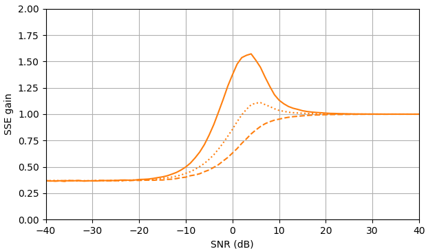
Figure 1. Monte Carlo estimations with a sample size of $10^5,$ of: Solid: gain of sum of square error in estimating $|X_k|$ by $\widehat{|X_k|}$ as compared to estimating it with $|Y_k|,$ dashed: gain of sum of square error in estimating $|X_k|^2$ by $\widehat{|X_k|^2}$ as compared to estimating it with $|Y_k|^2,$ dotted: gain of sum of square error in estimating $X_k$ by $\widehat{|X_k|}e^{i\arg(Y_k)}$ as compared to estimating it with $Y_k.$ The definition of $\widehat{|X_k|^2}$ from (3) is used.

Question: Is there another estimate of $|X_k|$ or $|X_k|^2$ that improves upon (2) and (3) without relying on the distribution of $Y_k$?

I think the problem is equivalent to estimating the square of the parameter $\displaystyle{\nu_\mathrm{Rice}}$ of a Rice distribution (Fig. 2) with known parameter $\sigma_\mathrm{Rice} = \frac{\sqrt{2}}{2}\sigma,$ given a single observation.

Figure 2. Rice distribution is the distribution of the distance $R$ to origin from a point that follows a bivariate circularly symmetric normal distribution with an absolute value of the mean $\nu_\mathrm{Rice},$ variance $2\sigma_\mathrm{Rice}^2 = \sigma^2$ and component variance $\sigma_\mathrm{Rice}^2 = \frac{1}{2}\sigma^2.$

I found some literature that seems relevant:

• Jan Sijbers, Arnold J. den Dekker, Paul Scheunders and Dirk Van Dyck, "Maximum Likelihood estimation of Rician distribution parameters", IEEE Transactions on Medical Imaging (Volume: 17, Issue: 3, June 1998) (doi, pdf).

Python script A for estimator curves

This script can be extended for plotting estimator curves in the answers.

import numpy as np
from mpmath import mp
import matplotlib.pyplot as plt

def plot_est(ms, est_as):
    fig = plt.figure(figsize=(4,4))
    ax = fig.add_subplot(1, 1, 1)
    if len(np.shape(est_as)) == 2:
        for i in range(np.shape(est_as)[0]):
            plt.plot(ms, est_as[i])
    else:
        plt.plot(ms, est_as)    
    plt.axis([ms[0], ms[-1], ms[0], ms[-1]])
    if ms[-1]-ms[0] < 5:
        ax.set_xticks(np.arange(np.int(ms[0]), np.int(ms[-1]) + 1, 1))
        ax.set_yticks(np.arange(np.int(ms[0]), np.int(ms[-1]) + 1, 1))
    plt.grid(True)
    plt.xlabel('$m$')
    h = plt.ylabel('$\hat a$')
    h.set_rotation(0)
    plt.show()

Python script B for Fig. 1

This script can be extended for error gain curves in the answers.

import math
import numpy as np
import matplotlib.pyplot as plt

def est_a_sub_fast(m):
    if m > 1:
        return np.sqrt(m*m - 1)
    else:
        return 0

def est_gain_SSE_a(est_a, a, N):
    SSE = 0
    SSE_ref = 0
    for k in range(N):  #Noise std. dev = 1, |X_k| = a
        m = abs(complex(np.random.normal(a, np.sqrt(2)/2), np.random.normal(0, np.sqrt(2)/2)))
        SSE += (a - est_a(m))**2 
        SSE_ref += (a - m)**2
    return SSE/SSE_ref

def est_gain_SSE_a2(est_a, a, N):
    SSE = 0
    SSE_ref = 0
    for k in range(N):  #Noise std. dev = 1, |X_k| = a
        m = abs(complex(np.random.normal(a, np.sqrt(2)/2), np.random.normal(0, np.sqrt(2)/2)))
        SSE += (a**2 - est_a(m)**2)**2
        SSE_ref += (a**2 - m**2)**2
    return SSE/SSE_ref

def est_gain_SSE_complex(est_a, a, N):
    SSE = 0
    SSE_ref = 0
    for k in range(N):  #Noise std. dev = 1, X_k = a
        Y = complex(np.random.normal(a, np.sqrt(2)/2), np.random.normal(0, np.sqrt(2)/2))        
        SSE += abs(a - est_a(abs(Y))*Y/abs(Y))**2
        SSE_ref += abs(a - Y)**2
    return SSE/SSE_ref

def plot_gains_SSE(as_dB, gains_SSE_a, gains_SSE_a2, gains_SSE_complex, color_number = 0):    
    colors = plt.rcParams['axes.prop_cycle'].by_key()['color']
    fig = plt.figure(figsize=(7,4))
    ax = fig.add_subplot(1, 1, 1)
    if len(np.shape(gains_SSE_a)) == 2:
        for i in range(np.shape(gains_SSE_a)[0]):
            plt.plot(as_dB, gains_SSE_a[i], color=colors[i], )
            plt.plot(as_dB, gains_SSE_a2[i], color=colors[i], linestyle='--')
            plt.plot(as_dB, gains_SSE_complex[i], color=colors[i], linestyle=':')
    else:
        plt.plot(as_dB, gains_SSE_a, color=colors[color_number])
        plt.plot(as_dB, gains_SSE_a2, color=colors[color_number], linestyle='--')
        plt.plot(as_dB, gains_SSE_complex, color=colors[color_number], linestyle=':')
    plt.grid(True)
    plt.axis([as_dB[0], as_dB[-1], 0, 2])
    plt.xlabel('SNR (dB)')
    plt.ylabel('SSE gain')
    plt.show()

as_dB = range(-40, 41)
as_ = [10**(a_dB/20) for a_dB in as_dB]
gains_SSE_a_sub = [est_gain_SSE_a(est_a_sub_fast, a, 10**5) for a in as_]
gains_SSE_a2_sub = [est_gain_SSE_a2(est_a_sub_fast, a, 10**5) for a in as_]
gains_SSE_complex_sub = [est_gain_SSE_complex(est_a_sub_fast, a, 10**5) for a in as_]

plot_gains_SSE(as_dB, gains_SSE_a_sub, gains_SSE_a2_sub, gains_SSE_complex_sub, 1)

Answer 1

Maximum likelihood (ML) estimator

Here will be derived a maximum-likelihood estimator of the power of the clean signal, but it doesn't seem to be improving things in terms of root mean square error, for any SNR, compared to spectral power subtraction.

Introduction

Let's introduce the normalized clean amplitude $a$ and normalized noisy magnitude $m$ normalized by the noise standard deviation $\sigma:$

$$a = \frac{|X_k|}{\sigma},\quad m = \frac{|Y_k|}{\sigma}.\tag{1}$$

The estimator in Eq. 3 of the question gives an estimate $\hat a$ of $a$ as:

$$\hat a = \frac{1}{\sigma}\sqrt{\widehat{|X_k|^2}} = \frac{1}{\sigma}\sqrt{\max\left((\sigma m)^2 - \sigma^2, 0\right)} = \cases{\sqrt{m^2-1}&if $m > 1,$\\0&if $m \le 1.$}\tag{2}$$

Maximum likelihood estimator

To make a possibly better estimator of $a$ than Eq. 2, we follow the procedure of Sijbers et al. 1998. (see question) to construct a maximum-likelihood (ML) estimator $\hat{a}_\mathrm{ML}.$ It gives the value of $a$ that maximizes the probability of the given value of $m.$

The PDF of $|Y_k|$ is Rician with parameter $\nu_\mathrm{Rice} = |X_k|$ and parameter (to be substituted later for clarity) $\sigma_\mathrm{Rice} = \frac{1}{\sqrt{2}}\sigma:$

$$\mathrm{PDF}(|Y_k|) = \frac{|Y_k|}{\sigma_\mathrm{Rice}^2}\exp\left(\frac{-\left(|Y_k|^2 + |X_k|^2\right)}{2\sigma_\mathrm{Rice}^2}\right)I_0\left(\frac{|Y_k||X_k|}{\sigma_\mathrm{Rice}^2}\right),\tag{3}$$

where $I_\alpha$ is a modified Bessel function of the first kind. Substituting $|X_k| = \sigma a,$ $|Y_k| = \sigma m,$ and $\sigma_\mathrm{Rice}^2 = \frac{1}{2}\sigma^2:$

$$= \mathrm{PDF}(\sigma m) = \frac{2m}{\sigma}e^{-\left(m^2 + a^2\right)}I_0(2ma),\tag{3.1}$$

and transforming:

$$\Rightarrow \mathrm{PDF}(m) = \sigma\mathrm{PDF}(\sigma m) = 2m e^{-\left(m^2 + a^2\right)}I_0(2ma).\tag{3.2}$$

The Rician PDF of $m$ parameterized by $a$ is independent of noise variance $\sigma^2.$ The maximum likelihood estimator $\hat a_\mathrm{ML}$ of parameter $a$ is the value of $a$ that maximizes $\mathrm{PDF}(m)$. It is a solution of:

$$m\frac{I_1(2m\hat a_\mathrm{ML})}{I_0(2m\hat a_\mathrm{ML})} - \hat a_\mathrm{ML} = 0.\tag{4}$$

The solution to Eq. 4 has the property that:

$$\hat a_\mathrm{ML} = 0\quad\text{ if }\quad m \le 1.\tag{5}$$

Otherwise it needs to be solved numerically.

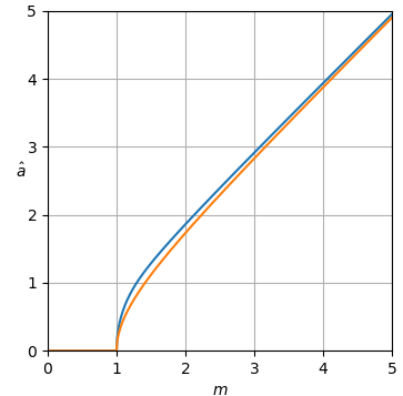
Figure 1. blue, upper: the maximum likelihood estimator $\hat a_\mathrm{ML}$ and orange, lower: the question's power spectral subtraction estimator $\hat a$ of normalized clean amplitude $a$, as function of normalized noisy magnitude $m.$

$\sigma\hat a_\mathrm{ML}$ is the maximum likelihood estimator of $|X_k|,$ and by functional invariance of maximum likelihood estimation, $\sigma^2\hat a_\mathrm{ML}^2$ is the maximum likelihood estimator of $|X_k|^2.$

Empirical Laurent series of the ML estimator

I tried to calculate numerically (see script further below) the Laurent series of $\hat a_\mathrm{ML}^2,$ but it does not seem to converge for the range of $m$ needed. Here is a truncation of the Laurent series as a far as I calculated it:

$$\hat a_\mathrm{ML}^2 \approx m^2 - \frac{1}{2^1m^0} - \frac{1}{2^3m^2} - \frac{3}{2^5m^4} - \frac{12}{2^7m^6} - \frac{57}{2^9m^8} - \frac{309}{2^{11}m^{10}} - \frac{1884}{2^{13}m^{12}} - \frac{12864}{2^{15}m^{14}} - \frac{98301}{2^{17}m^{16}} - \frac{839919}{2^{19}m^{18}} - \frac{7999311}{2^{21}m^{20}}\tag{6}$$

I could not find the numerator or denominator integer sequences in the On-line Encyclopedia of Integer Sequences (OEIS). Only for the first five negative-power terms, the numerator coefficients match with A027710. However, after submitting the computed sequence ($1, -1, -1, -3, \ldots$) to OEIS Superseeker, I got this in the reply (from which I confirmed the next three suggested numbers $-84437184, -980556636, -12429122844$ by an extended calculation):

Guesss suggests that the generating function  F(x)
may satisfy the following algebraic or differential equation:

-1/2*x+1/2+(-x+1/2)*x*diff(F(x),x)+(x-3/2)*F(x)-1/2*F(x)*x*diff(F(x),x)+F(x)^2 = 0

If this is correct the next 6 numbers in the sequence are:

[-84437184, -980556636, -12429122844, -170681035692, -2522486871192, -39894009165525]

Tabulated approximation and estimation error gain

A linearly interpolated table (see scripts below) containing $124071$ non-uniformly distributed samples of $\hat a_\mathrm{ML}^2-m^2$ gives an approximation with a maximum error of about $6\times10^{-11}.$

Least squares approximation of the ML estimator

A least squares approximation (with extra weight at $m^2 = 1$) of the samples of the estimator curve was created, in form inspired by the Laurent series experiments (see Octave script further down). The constant term - 0.5 was changed to - 0.49999998237308493999 to remove the possibility of negative $a^2$ at $m^2 = 1.$ The approximation is valid for $m^2 \ge 1$ and has a maximum error of about $2\times10^{-5}$ (Fig. 3) in approximating $\hat a_\mathrm{ML}^2:$

a^2 = m^2 - 0.49999998237308493999 -0.1267853520007855/m^2 - 0.02264263789612356/m^4 - 1.008652066326489/m^6 + 4.961512935048501/m^8 - 12.27301424767318/m^10 + 5.713416605734312/m^12 + 21.55623892529696/m^14 - 38.15890985013438/m^16 + 24.77625343690267/m^18 - 5.917417766578400/m^20

Figure 3. Error of the least squares approximation of $\hat a_\mathrm{ML}^2.$

The script seems capable of handling increasing the number of negative powers of $m^2,$ consistently giving smaller and smaller errors, with the number of error extrema growing, but with quite a slow maximum error decay. The approximation is almost equiripple, but would still benefit a bit from Remez exchange refinement.

Using the approximation, the following expected error gain curves were obtained:

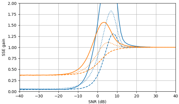
Figure 2. Monte Carlo estimations with a sample size of $10^5,$ of: Solid: gain of sum of square error in estimating $|X_k|$ by $\widehat{|X_k|}$ as compared to estimating it with $|Y_k|,$ dashed: gain of sum of square error in estimating $|X_k|^2$ by $\widehat{|X_k|^2}$ as compared to estimating it with $|Y_k|^2,$ dotted: gain of sum of square error in estimating $X_k$ by $\widehat{|X_k|}e^{i\arg(Y_k)}$ as compared to estimating it with $Y_k.$ Blue: ML estimator, orange: clamped spectral power subtraction.

Surprisingly, the ML estimator is worse than clamped spectral power subtraction in almost all aspects, except for being marginally better for signal estimation at SNR > about 5 dB, and amplitude estimation at SNR > about 3 dB. At those SNR, the two estimators are worse than just using the noisy signal as the estimate.

Python script A for Fig. 1

This script extends the question's script A.

def est_a_sub(m):
    m = mp.mpf(m)
    if m > 1:
        return mp.sqrt(m**2 - 1)
    else:
        return 0

def est_a_ML(m):
    m = mp.mpf(m)
    if m > 1:
        return mp.findroot(lambda a: m*mp.besseli(1, 2*a*m)/(mp.besseli(0, 2*a*m)) - a, [mp.sqrt(2*m**2*(m**2 - 1)/(2*m**2 - 1)), mp.sqrt(m**2-0.5)])
    else:
        return 0

def est_a_ML_fast(m): 
    m = mp.mpf(m)
    if m > 1:
        return mp.sqrt(m**2 - mp.mpf('0.49999998237308493999') - mp.mpf('0.1267853520007855')/m**2 - mp.mpf('0.02264263789612356')/m**4 - mp.mpf('1.008652066326489')/m**6 + mp.mpf('4.961512935048501')/m**8 - mp.mpf('12.27301424767318')/m**10 + mp.mpf('5.713416605734312')/m**12 + mp.mpf('21.55623892529696')/m**14 - mp.mpf('38.15890985013438')/m**16 + mp.mpf('24.77625343690267')/m**18 - mp.mpf('5.917417766578400')/m**20)
    else:
        return 0

ms = np.arange(0, 5.0078125, 0.0078125)
est_as = [[est_a_ML(m) for m in ms], [est_a_sub(m) for m in ms]];
plot_est(ms, est_as)

Python script for numerical calculation of Laurent series

This script calculates numerically the first few terms of the Laurent series of $\hat a_\mathrm{ML}^2-m^2.$ It is based on the script in this answer.

from sympy import *
from mpmath import *
num_terms = 10
num_decimals = 12
num_use_decimals = num_decimals + 5 #Ad hoc headroom
def y(a2):
    return sqrt(m2)*besseli(1, 2*sqrt(a2*m2))/besseli(0, 2*sqrt(a2*m2)) - sqrt(a2)

c = []
h = mpf('1e'+str(num_decimals))
denominator = mpf(2)  # First integer denominator. Use 1 if unsure
denominator_ratio = 4  # Denominator multiplier per step. Use 1 if unsure
print("x")
for i in range(0, num_terms):
    mp.dps = 2*2**(num_terms - i)*num_use_decimals*(i + 2) #Ad hoc headroom
    m2 = mpf('1e'+str(2**(num_terms - i)*num_use_decimals))
    r = findroot(y, [2*m2*(m2 - 1)/(2*m2 - 1),  m2-0.5]) #Safe search range, must be good for the problem
    r = r - m2; # Part of the problem definition
    for j in range(0, i):
        r = (r - c[j])*m2
    c.append(r)
    mp.dps = num_decimals
    print '+'+str(nint(r*h)*denominator/h)+'/('+str(denominator)+'x^'+str(i)+')'
    denominator *= denominator_ratio

Python script for tabulation of the ML estimator

This script creates an unevenly sampled table of $\left[m^2, \hat{a}_\mathrm{ML}^2\right]$ pairs suitable for linear interpolation, giving approximately the defined maximum absolute linear interpolation error of approximating $\hat{a}_\mathrm{ML}^2$ for the range $m = 0\ldots m_\max.$ The table size is automatically increased by adding samples to the difficult parts, until the peak error is small enough. If $m_\max$ equals $2$ plus an integer power of $2,$ then all sampling intervals will be powers of $2.$ At the end of the table there will be a discontinuity-free transition to a large-$m$ approximation $\hat{a}_\mathrm{ML}^2 = m^2 - \frac{1}{2}.$ If $\hat{a}_\mathrm{ML}$ is needed, my guess is that it is better to interpolate the table as is and then do the conversion $\hat{a}_\mathrm{ML} = \sqrt{\hat{a}_\mathrm{ML}^2}.$

For use in conjunction with the next script, pipe the output > linear.m.

import sys # For writing progress to stderr (won't pipe when piping output to a file)
from sympy import *
from mpmath import *
from operator import itemgetter
max_m2 = 2 + mpf(2)**31 # Maximum m^2
max_abs_error = 2.0**-34 #Maximum absolute allowed error in a^2
allow_over = 0 #Make the created samples have max error (reduces table size to about 7/10)
mp.dps = 24
print('# max_m2='+str(max_m2))
print('# max_abs_error='+str(max_abs_error))
def y(a2):
    return sqrt(m2)*besseli(1, 2*sqrt(a2*m2))/besseli(0, 2*sqrt(a2*m2)) - sqrt(a2)

# [m2, a2, following interval tested good]
samples = [[0, 0, True], [1, 0, False], [max_m2, max_m2 - 0.5, True]]

m2 = mpf(max_m2)
est_a2 = findroot(y, [2*m2*(m2 - 1)/(2*m2 - 1),  m2-0.5])
abs_error = abs(est_a2 - samples[len(samples) - 1][1])
if abs_error > max_abs_error:
    sys.stderr.write('increase max_m, or increase max_abs_error to '+str(abs_error)+'\n')
    quit()

peak_taken_abs_error = mpf(max_abs_error*allow_over)
while True:
    num_old_samples = len(samples)
    no_new_samples = True
    peak_trial_abs_error = peak_taken_abs_error
    for i in range(num_old_samples - 1):
        if samples[i][2] == False:
            m2 = mpf(samples[i][0] + samples[i + 1][0])/2
            est_a2 = mpf(samples[i][1] + samples[i + 1][1])/2
            a2 = findroot(y, [2*m2*(m2 - 1)/(2*m2 - 1),  m2-0.5])
            est_abs_error = abs(a2-est_a2)
            if peak_trial_abs_error < est_abs_error:
                peak_trial_abs_error = est_abs_error
            if est_abs_error > max_abs_error:                
                samples.append([m2, a2 + max_abs_error*allow_over, False])
                no_new_samples = False
            else:
                samples[i][2] = True
                if peak_taken_abs_error < est_abs_error:
                    peak_taken_abs_error = est_abs_error
    if no_new_samples == True:
        sys.stderr.write('error='+str(peak_taken_abs_error)+', len='+str(len(samples))+'\n')
        print('# error='+str(peak_taken_abs_error)+', len='+str(len(samples)))
        break
    sys.stderr.write('error='+str(peak_trial_abs_error)+', len='+str(len(samples))+'\n')
    samples = sorted(samples, key=itemgetter(0))

print('global m2_to_a2_table = [')
for i in range(len(samples)):
    if i < len(samples) - 1:
      print('['+str(samples[i][0])+', '+str(samples[i][1])+'],')
    else:
      print('['+str(samples[i][0])+', '+str(samples[i][1])+']')
print('];')

Python script B for Fig. 2

This script extends the question's script B.

def est_a_ML_fast(m): 
    mInv = 1/m
    if m > 1:
        return np.sqrt(m**2 - 0.49999998237308493999 - 0.1267853520007855*mInv**2 - 0.02264263789612356*mInv**4 - 1.008652066326489*mInv**6 + 4.961512935048501*mInv**8 - 12.27301424767318*mInv**10 + 5.713416605734312*mInv**12 + 21.55623892529696*mInv**14 - 38.15890985013438*mInv**16 + 24.77625343690267*mInv**18 - 5.917417766578400*mInv**20)
    else:
        return 0

gains_SSE_a_ML = [est_gain_SSE_a(est_a_ML_fast, a, 10**5) for a in as_]
gains_SSE_a2_ML = [est_gain_SSE_a2(est_a_ML_fast, a, 10**5) for a in as_]
gains_SSE_complex_ML = [est_gain_SSE_complex(est_a_ML_fast, a, 10**5) for a in as_]
plot_gains_SSE(as_dB, [gains_SSE_a_ML, gains_SSE_a_sub], [gains_SSE_a2_ML, gains_SSE_a2_sub], [gains_SSE_complex_ML, gains_SSE_complex_sub])

Octave script for least squares

This Octave script (an adaptation of this answer) does a least squares fit of powers of $m^2$ into $\hat{a}_\mathrm{ML}^2 - (m^2 - \frac{1}{2})$. The samples were prepared by the Python script a bit above.

graphics_toolkit("fltk");
source("linear.m");
format long
dup_zero = 2000000  # Give extra weight to m2 = 1, a2 = 0
max_neg_powers = 10  # Number of negative powers in the polynomial
m2 = m2_to_a2_table(2:end-1,1);
m2 = vertcat(repmat(m2(1), dup_zero, 1), m2);
A = (m2.^-[1:max_neg_powers]);
a2_target = m2_to_a2_table(2:end-1,2);
a2_target = vertcat(repmat(a2_target(1), dup_zero, 1), a2_target);
fun_target = a2_target - m2 + 0.5;
disp("Cofficients for negative powers of m^2:")
x = A\fun_target
a2 = A*x + m2 - 0.5;
plot(sqrt(m2), sqrt(a2)) # Plot approximation
xlim([0, 3])
ylim([0, 3])
a2(1)  # value at m2 = 2
abs_residual = abs(a2-a2_target);
max(abs_residual) # Max abs error of a^2
max(abs(sqrt(a2)-sqrt(a2_target))) # Max abs error of a
plot(sqrt(log10(m2)), a2_target - a2) # Plot error
xlabel("sqrt(log(m^2))")
ylabel("error in approximation of hat a^2_{ML}")

Python script A2 for approximation using Chebyshev polynomials

This script extends script A and gives an alternative approximation of the ML estimator using Chebyshev polynomials. The first Chebyshev node is at $m=1$ and the number of Chebyshev polynomials is such that the approximation is nonnegative.

N = 20
est_a_ML_poly, err = mp.chebyfit(lambda m2Reciprocal: est_a_ML(mp.sqrt(1/m2Reciprocal))**2 - 1/m2Reciprocal, [0, 2/(mp.cos(mp.pi/(2*N)) + 1)], N, error=True)

def est_a_ML_fast(m): 
    global est_a_ML_poly
    m = mp.mpf(m)
    if m > 1:
        return mp.sqrt(m**2 + mp.polyval(est_a_ML_poly, 1/m**2))
    else:
        return 0

Answer 2

Update:

I'm sorry to have to say that testing shows the following argument seems to break down under heavy noise. This is not what I expected, so I have definitely learned something new. My prior testing had all been in the high SNR range as my focus has been on finding exact solutions in the noiseless case.

---

Olli,

If your goal is to find the parameters of a pure tone in a noisy signal, you should have said so. This issue, I have lots of experience and expertise in.

You say you are looking for the amplitude (and phase comes with it) so I bet you are lining up your DFT to have a whole number of cycles. This is the worst configuration for this situation as you are then dealing with your signal in just a single bin against the noise in that single bin.

As you have shown above, the greater the SNR the worse your trick performs, to the point of detrimental or beyond. Well, your bin of interest is going to be the one with the highest SNR.

What you want to do is align your DFT frame on a whole plus one half cycle. This will spread your signal across as many bins as possible. Then you can find the phase and amplitude as described in my blog article on the topic Phase and Amplitude Calculation for a Pure Real Tone in a DFT: Method 1.

In short, you treat the set of bins near the peak as a complex vector space. Then knowing the frequency, you construct a set of basis vectors for your signal. The coefficients of the vectors act as a virtual bin which will tell you the amplitude of the signal as well as the phase. By finding the best fit vector across several bins, the technique does not allow the noise in any given bin to be too dominant and sort of provides a "lever" that the noise has to balance around. The noise reduction effects are similar to when random variables are averaged together.

Constructing the basis vectors means taking the DFT of a sine and cosine at your frequency. I have a formula for their direct calculation which bypasses having to do a summation. The article for that is linked from the above article.

I would be interested in finding out if your technique does improve the results of this method. I am used to working in higher SNR >> 1 so I have never really tested at the noise levels you are dealing with.

Synopsis of the approach:

$$ x[n] = a \cdot \cos( \omega n ) + b \cdot \sin( \omega n ) + wgn[n] $$

Because the DFT is a linear operator:

$$ DFT( x[n] ) = a \cdot DFT( \cos( \omega n ) ) + b \cdot DFT( \sin( \omega n ) ) + DFT( wgn[n] ) $$

In vector notation:

$$ Z = a \cdot A + b \cdot B + W $$

You are simply solving for $a$ and $b$ using standard linear algebra to give you a best fit. A bonus is that you also get an estimate of W. Therefore, you can try a "throw the bum out" approach, and completely eliminate the estimated noise in the worst fitting bin and then recalculate. Rinse, repeat. Or reduce the noise in each bin by some other formula. If you do it proportionally, your results will remain the same as W is orthogonal to A and B. But a constant subtraction along W, rather than Z (as your method does) should improve results as well.

Normally, I do the four bins around the peak, but you might want to extend that to 6 or even 8. At some point, more bins makes for worse results as you are bringing in more noise than signal.

You only have to calculate the DFT bins of interest.

Answer 3

An interesting approximative solution of the maximum likelihood (ML) estimation problem is obtained by using the asymptotic formula

$$I_0(x)\approx \frac{e^x}{\sqrt{2\pi x}},\qquad x\gg 1\tag{1}$$

Using the notation and formulas from Olli's answer, the optimum ML estimate of the normalized clean signal amplitude satisfies

$$\hat{a}=m\frac{I_1(2m\hat{a})}{I_0(2m\hat{a})}\tag{2}$$

Using $(1)$ and noting that $I_1(x)=I_0'(x)$, we obtain the approximation

$$\frac{I_1(x)}{I_0(x)}\approx 1-\frac{1}{2x}\tag{3}$$

This approximation has a relative error of less than $1$% for $x>4.5$.

Plugging $(3)$ into $(2)$ gives the approximative solution

$$\hat{a}\approx\frac12\left(m+\sqrt{m^2-1}\right)\tag{4}$$

With $m=|Y_k|/\sigma$ and $a=|X_k|/\sigma$ we obtain

$$\widehat{|X|_k}\approx\frac12\left(|Y_k|+\sqrt{|Y_k|^2-\sigma^2}\right)\tag{5}$$

which is simply the arithmetic mean of the noisy observation $|Y_k|$ and the estimate obtained from spectral power subtraction.

---

EDIT:

I would be nice to have an approximation like $(3)$ that works over the whole range $x\in[0,\infty)$. A candidate for such an approximation is the family of functions

$$f(x)=\frac{x}{\sqrt{c_1+c_2x^2}}\tag{6}$$

The theoretically correct choice of the constants is $c_1=4$ and $c_2=1$, considering the properties of $f(x)$ around $x=0$ and $x\rightarrow\infty$. However, for a realistic range of $x$, a better approximation in that range might be achievable by tweaking those constants a bit.

Using the approximation $(6)$ with $c_1=4$ and $c_2=1$ results in the following estimate:

$$\hat{a}=m\sqrt{1-\frac{1}{m^4}}\tag{7}$$

or, equivalently,

$$\widehat{|X|_k}=|Y_k|\sqrt{1-\frac{\sigma^4}{|Y_k|^4}}\tag{8}$$

---

Olli's edit:

Figure 1. $\hat a_\text{ML}$ (orange) and its approximations defined by Eq. 4 (blue) and Eq. 7 (green), as function of $m.$ All curves approach $a = m$ as $m\to\infty$ (see right figure for large $m$). $\hat a_\text{ML}^2$ asymptotically approaches its truncated Laurent series $m^2-\frac{1}{2}$ as $m\to\infty,$ which gives the curious result that even though the approximations of $\hat a_\text{ML}$ asymptotically approach it as $m\to\infty$, the square of Eq. 7 has constant error in approximating $\hat a_\text{ML}^2$ as $m\to\infty$ because the constant term 0 of its Laurent series differs from $-\frac{1}{2}$ of the Laurent series of $\hat a_\text{ML}^2$ (see Olli's ML estimator answer) and the Laurent series of the square of Eq. 4. This constant error $c$ disappears in estimation of $\hat a_\text{ML}$ due to the fact that $\lim_{m\to\infty}\left(\sqrt{m^2 + c} - m\right) = 0.$

Python script for Fig. 1

This script requires the question's script for module imports and for the plotting function plot_est, and the function definition of est_a_ML from Olli's ML answer.

def est_a_MattL_Eq_4(m):
    m = mp.mpf(m)
    if m > 1:
        return (m + mp.sqrt(m**2 - 1))/2
    else:
        return 0

def est_a_MattL_Eq_7(m):
    m = mp.mpf(m)
    if m > 1:
        return m*mp.sqrt(1 - 1/m**4)
    else:
        return 0

ms = np.arange(0, 2.00390625, 0.00390625)
est_as = [[est_a_MattL_Eq_4(m) for m in ms], [est_a_ML(m) for m in ms], [est_a_MattL_Eq_7(m) for m in ms]];
plot_est(ms, est_as)

ms = np.arange(18, 20.125, 0.125)
est_as = [[est_a_MattL_Eq_4(m) for m in ms], [est_a_ML(m) for m in ms], [est_a_MattL_Eq_7(m) for m in ms]];
plot_est(ms, est_as)

Answer 4

Scale-invariant minimum mean square error (MMSE) improper uniform prior estimators of transformed amplitude

This answer presents a family scale-invariant estimators, parameterized by a single parameter which controls both the Bayesian prior distribution of amplitude and the transformation of amplitude to another scale. The estimators are minimum mean square error (MMSE) estimators in the transformed amplitude scale. An improper uniform prior of transformed amplitude is assumed. Available transformations include a linear scale (no transformation) and can approach a logarithmic scale whereby the estimator approaches zero everywhere. The estimators can be parameterized to attain low sum of square error at negative signal-to-noise ratios (SNRs).

Bayesian estimation

The maximum likelihood (ML) estimator in my first answer performed rather poorly. The ML estimator can also be understood as a Bayesian maximum a posteriori (MAP) estimator given an improper uniform prior probability distribution. Here, improper means that the prior extends from zero to infinity with infinitesimal density. Because the density is not a real number, the prior is not a proper distribution, but it may still give a proper posterior distribution by Bayes' theorem which can then be used to obtain a MAP or an MMSE estimate.

They Bayes' theorem in terms of probability density functions (PDFs) is:

$$\operatorname{PDF}(a\mid m) = \frac{\operatorname{PDF}(m\mid a)\,\operatorname{PDF}(a)}{\operatorname{PDF}(m)} = \frac{\operatorname{PDF}(m\mid a)\,\operatorname{PDF}(a)}{\int_0^\infty\operatorname{PDF}(m\mid a)\,\operatorname{PDF}(a)\,da}.\tag{1}$$

A MAP estimator $\hat a_\text{MAP}$ is the argument of the posterior PDF that maximizes it:

$$\hat a_\text{MAP} = \underset{a}{\operatorname{arg\,max}}\operatorname{PDF}(a \mid m).\tag{2}$$

An MMSE estimator $\hat a_\text{MMSE}$ is the posterior mean:

$$\hat a_\text{MMSE} = \underset{\hat a}{\operatorname{arg\,max}}\operatorname{E}[(a - \hat a)^2\mid m] = \operatorname{E}[a\mid m] = \int_0^\infty a \operatorname{PDF}(a\mid m)da.\tag{3}$$

An improper uniform prior is not the only scale-invariant prior. Any prior PDF satisfying:

$$\operatorname{PDF(|X_k|)} \propto |X_k|^{\varepsilon-1},\tag{4}$$

with real exponent $\varepsilon-1,$ and $\propto$ meaning: "is proportional to", is scale-invariant in the sense that the product of $X_k$ and a positive constant still follows the same distribution (see Lauwers et al. 2010).

A family of estimators

A family of estimators shall be presented, with these properties:

1. Scale-invariance: If the complex clean bin $X_k,$ or equivalently the clean amplitude $|X_k|,$ and the noise standard deviation $\sigma$ are each multiplied by the same positive constant, then also the estimated amplitude $\widehat{|X_k|}$ gets multiplied by that constant.
2. Minimum mean square transformed-amplitude error.
3. Improper uniform prior of transformed amplitude.

We shall use normalized notation:

$$\begin{array}{ll} a &= \frac{|X_k|}{\sigma}&\text{normalized clean amplitude,}\\ m &= \frac{|Y_k|}{\sigma}&\text{normalized noisy magnitude,}\\ 1 &= \left(\frac{\sigma}{\sigma}\right)^2&\text{normalized variance of noise,}\\ \mathrm{SNR} &= \left(\frac{|X_k|}{\sigma}\right)^2 = a^2&\text{signal-to-noise ratio ($10\log_{10}(\mathrm{SNR})$ dB),}\end{array}\tag{5}$$

where $|X_k|$ is the clean amplitude we wish to estimate from the noisy magnitude $|Y_k|$ of bin value $Y_k$ whicy equals the sum of clean bin value $X_k$ plus circularly symmetric complex Gaussian noise of variance $\sigma^2.$ The scale-invariant prior of $|X_k|$ given in Eq. 4 is carried over to the normalized notation as:

$$\operatorname{PDF}(a) \propto a^{\varepsilon - 1}.\tag{6}$$

Let $g(a)$ be an increasing transformation function of amplitude $a.$ The improper uniform prior of transformed amplitude is denoted by:

$$\operatorname{PDF}\big(g(a)\big) \propto 1.\tag{7}$$

Eqs. 6 & 7 together determine the family of possible amplitude transformations. They are related by a change of variables:

$$\begin{array}{rrcl}&g'(a) \operatorname{PDF}\big(g(a)\big) &=& \operatorname{PDF}(a)\\ \displaystyle\Rightarrow&\quad g'(a) &\propto& a^{\varepsilon - 1}\\ \Rightarrow&g(a) &\propto& \displaystyle\int a^{\varepsilon - 1} da = \frac{a^\varepsilon}{\varepsilon} + c\\ \Rightarrow&g(a) &=& \displaystyle\frac{c_1a^\varepsilon}{\varepsilon} + c_0.\end{array}\tag{8}$$

We assume without proof that the choice of the constants $c_0$ and $c_1$ will not affect the amplitude estimate. For convenience we set:

$$\begin{array}{rc}&g(1) = 1\quad\text{and}\quad g'(1) = 1\\ \Rightarrow&c_0 = \displaystyle\frac{\varepsilon - 1}{\varepsilon}\quad\text{and}\quad c_1 = 1\\ \Rightarrow&g(a) = \displaystyle\frac{a^\varepsilon + \varepsilon - 1}{\varepsilon},\\ \end{array}\tag{9}$$

which has a special linear case:

$$g(a) = a\quad\text{if}\quad \varepsilon = 1,\tag{10}$$

and a limit:

$$\lim_{\varepsilon \to 0}g(a) = \log(a) + 1.\tag{11}$$

The transformation function can conveniently represent the linear amplitude scale (at $\varepsilon = 1$) and can approach a logarithmic amplitude scale (as $\varepsilon \to 0$). For positive $\varepsilon,$ the support of the PDF of transformed amplitude is:

$$\begin{eqnarray}&0 < a < \infty&\\ \Rightarrow\quad&\frac{\varepsilon - 1}{\varepsilon} < g(a) < \infty,&\end{eqnarray}\tag{12}$$

The inverse transformation function is:

$$g^{-1}\big(g(a)\big) = \big(\varepsilon g(a) - \varepsilon + 1\big)^{1/\varepsilon} = a.\tag{13}$$

The transformed estimate is then, using the law of the unconscious statistician:

$$\begin{gather}\hat a_\text{uni-MMSE-xform} = \underset{\hat a}{\operatorname{arg\,min}}\operatorname{E}\left[\big(g(a) - g(\hat a)\big)^2\mid m\right] = g^{-1}\big(\operatorname{E}[g(a) \mid m]\big)\\ = g^{-1}\left(\int_0^\infty g(a) \operatorname{PDF}(a \mid m)\,da\right)\\ = g^{-1}\left(\frac{\int_0^\infty g(a) f(a \mid m)da}{\int_0^\infty f(a \mid m)da}\right),\end{gather}\tag{14}$$

where $\operatorname{PDF}(a \mid b)$ is the posterior PDF and $f(a \mid m)$ is an unnormalized posterior PDF defined using Bayes' theorem (Eq. 1), the Rician $\operatorname{PDF}(m \mid a) = 2me^{-\left(m^2 + a^2\right)}I_0(2ma)$ from Eq. 3.2 of my ML estimator answer, and Eq. 6:

$$\begin{eqnarray}\operatorname{PDF}(a\mid m) &\propto& \operatorname{PDF}(m\mid a)\,\operatorname{PDF}(a)\\ &\propto&2me^{-\left(m^2 + a^2\right)}I_0(2ma)\times a^{\varepsilon - 1}\\ &\propto&e^{-a^2}I_0(2ma)\,a^{\varepsilon - 1} = f(a \mid m),\end{eqnarray}\tag{15}$$

from which $\operatorname{PDF}(m)$ was dropped from the Bayes' formula because it is constant over $a.$ Combining Eqs. 14, 9 & 15, solving the integrals in Mathematica, and simplifying, gives:

$$\begin{gather}\hat a_\text{uni-MMSE-xform}=g^{-1}\left(\frac{\int_0^\infty \frac{a^\varepsilon + \varepsilon - 1}{\varepsilon} \times e^{-a^2}I_0(2ma)\,a^{\varepsilon - 1}\,da}{\int_0^\infty e^{-a^2}I_0(2ma)\,a^{\varepsilon - 1}\,da}\right)\\ = \left(\varepsilon\frac{\frac{1}{2\varepsilon}\left(\Gamma(\varepsilon) L_{-\varepsilon}(m^2) + (\varepsilon-1) \Gamma(\varepsilon/2) L_{-\varepsilon/2}(m^2)\right)}{\frac{1}{2} \Gamma(\varepsilon/2) L_{-\varepsilon/2}(m^2)} - \varepsilon + 1\right)^{1/\varepsilon}\\ = \left(\frac{\Gamma(\varepsilon) L_{-\varepsilon}(m^2) + (\varepsilon-1) \Gamma(\varepsilon/2) L_{-\varepsilon/2}(m^2)}{\Gamma(\varepsilon/2) L_{-\varepsilon/2}(m^2)} - \varepsilon + 1\right)^{1/\varepsilon}\\ = \left(\frac{\Gamma(\varepsilon) L_{-\varepsilon}(m^2)}{\Gamma(\varepsilon/2) L_{-\varepsilon/2}(m^2)}\right)^{1/\varepsilon},\end{gather}\tag{16}$$

where $\Gamma$ is the gamma function and $L$ is the Laguerre function. The estimator collapses to zero everywhere as $\varepsilon \to 0,$ so it does not make sense to use negative $\varepsilon,$ which would emphasis small values of $a$ even further and give an improper posterior distribution. Some special cases are:

$$\hat a_\text{uni-MMSE-xform} = \sqrt{m^2 + 1},\quad\text{if }\varepsilon = 2,\tag{17}$$

$$\hat a_\text{uni-MMSE} = \hat a_\text{uni-MMSE-xform}= \frac{e^{m^2/2}}{\sqrt{\pi} I_0(m^2/2)},\quad\text{if }\varepsilon = 1,\tag{18}$$

approximated at large $m$ by (see calculation) a truncated Laurent series:

$$\hat a_\text{uni-MMSE} \approx m - \frac{1}{4m} - \frac{7}{32m^3} - \frac{59}{128m^5},\tag{19}$$

This asymptotic approximation has an absolute maximum amplitude error of less than $10^{-6}$ for $m > 7.7.$

The estimator curves are shown in Fig. 1.

Figure 1. Estimator $\hat a_\text{uni-MMSE-xform}$ as function of $m$ for different values of $\varepsilon,$ from top to bottom: blue: $\varepsilon = 2,$ which minimizes the mean square power error assuming an improper uniform prior of power, orange: $\varepsilon = 1,$ which minimizes the mean square amplitude error assuming an improper uniform prior of amplitude, green: $\varepsilon = \frac{1}{2},$ red: $\varepsilon = \frac{1}{4},$ and purple: $\varepsilon = \frac{1}{8}.$

At $m=0$ the curves are horizontal with value:

$$\hat a_\text{uni-MMSE-xform} = \frac{2^{1 - 1/\varepsilon} \bigg(\Gamma\Big(\frac{1 + \varepsilon}{2}\Big)\bigg)^{1/\varepsilon}}{\pi^{1/(2\varepsilon)}},\quad\text{if }m = 0.\tag{20}$$

At negative SNR, the uni-MMSE-xform estimator can be parameterized using low $\varepsilon$ to give a lower sum of square error compared to the clamped spectral power subtraction estimator, with a corresponding penalty at intermediate SNR values near 7 dB (Fig. 2).

Figure 2. Monte Carlo estimations with a sample size of $10^5,$ of: Solid: gain of sum of square error in estimating $|X_k|$ by $\widehat{|X_k|}$ as compared to estimating it with $|Y_k|,$ dashed: gain of sum of square error in estimating $|X_k|^2$ by $\widehat{|X_k|^2}$ as compared to estimating it with $|Y_k|^2,$ dotted: gain of sum of square error in estimating $X_k$ by $\widehat{|X_k|}e^{i\arg(Y_k)}$ as compared to estimating it with $Y_k.$ Blue: uni-MMSE-xform estimator with $\varepsilon = 1$ (top), $\varepsilon = \frac{1}{2}$ (middle), and $\varepsilon = \frac{1}{4},$ orange: clamped spectral power subtraction.

Python script for Fig. 1

This script extends the question's script A.

def est_a_uni_MMSE_xform(m, epsilon):
    m = mp.mpf(m)
    epsilon = mp.mpf(epsilon)
    if epsilon == 0:
        return mpf(0)
    elif epsilon == 1:
        return mp.exp(m**2/2)/(mp.sqrt(mp.pi)*mp.besseli(0, m**2/2))
    elif epsilon == 2:
        return mp.sqrt(m**2 + 1)
    else:
        return (mp.gamma(epsilon)*mp.laguerre(-epsilon, 0, m**2) / (mp.gamma(epsilon/2)*mp.laguerre(-epsilon/2, 0, m**2)))**(1/epsilon)

ms = np.arange(0, 6.0625, 0.0625)
est_as_uni_MMSE_xform = [[est_a_uni_MMSE_xform(m, 2) for m in ms], [est_a_uni_MMSE_xform(m, 1) for m in ms], [est_a_uni_MMSE_xform(m, 0.5) for m in ms], [est_a_uni_MMSE_xform(m, 0.25) for m in ms],  [est_a_uni_MMSE_xform(m, 0.125) for m in ms]]
plot_est(ms, est_as_uni_MMSE_xform)

Python script for Fig. 2

This script extends the question's script B. The function est_a_uni_MMSE_xform_fast may be numerically unstable.

from scipy import special

def est_a_uni_MMSE_fast(m):
    return 1/(np.sqrt(np.pi)*special.i0e(m**2/2))

def est_a_uni_MMSE_xform_fast(m, epsilon):
    if epsilon == 0:
        return 0
    elif epsilon == 1:
        return 1/(np.sqrt(np.pi)*special.i0e(m**2/2))
    elif epsilon == 2:
        return np.sqrt(m**2 + 1)
    else:
        return (special.gamma(epsilon)*special.eval_laguerre(-epsilon, m**2)/(special.gamma(epsilon/2)*special.eval_laguerre(-epsilon/2, m**2)))**(1/epsilon)

gains_SSE_a_uni_MMSE = [est_gain_SSE_a(est_a_uni_MMSE_fast, a, 10**5) for a in as_]
gains_SSE_a2_uni_MMSE = [est_gain_SSE_a2(est_a_uni_MMSE_fast, a, 10**5) for a in as_]
gains_SSE_complex_uni_MMSE = [est_gain_SSE_complex(est_a_uni_MMSE_fast, a, 10**5) for a in as_]
plot_gains_SSE(as_dB, [gains_SSE_a_uni_MMSE, gains_SSE_a_sub], [gains_SSE_a2_uni_MMSE, gains_SSE_a2_sub], [gains_SSE_complex_uni_MMSE, gains_SSE_complex_sub])

gains_SSE_a_uni_MMSE_xform_0e5 = [est_gain_SSE_a(lambda m: est_a_uni_MMSE_xform_fast(m, 0.5), a, 10**5) for a in as_]
gains_SSE_a2_uni_MMSE_xform_0e5 = [est_gain_SSE_a2(lambda m: est_a_uni_MMSE_xform_fast(m, 0.5), a, 10**5) for a in as_]
gains_SSE_complex_uni_MMSE_xform_0e5 = [est_gain_SSE_complex(lambda m: est_a_uni_MMSE_xform_fast(m, 0.5), a, 10**5) for a in as_]
plot_gains_SSE(as_dB, [gains_SSE_a_uni_MMSE_xform_0e5, gains_SSE_a_sub], [gains_SSE_a2_uni_MMSE_xform_0e5, gains_SSE_a2_sub], [gains_SSE_complex_uni_MMSE_xform_0e5, gains_SSE_complex_sub])

gains_SSE_a_uni_MMSE_xform_0e25 = [est_gain_SSE_a(lambda m: est_a_uni_MMSE_xform_fast(m, 0.25), a, 10**5) for a in as_]
gains_SSE_a2_uni_MMSE_xform_0e25 = [est_gain_SSE_a2(lambda m: est_a_uni_MMSE_xform_fast(m, 0.25), a, 10**5) for a in as_]
gains_SSE_complex_uni_MMSE_xform_0e25 = [est_gain_SSE_complex(lambda m: est_a_uni_MMSE_xform_fast(m, 0.25), a, 10**5) for a in as_]
plot_gains_SSE(as_dB, [gains_SSE_a_uni_MMSE_xform_0e25, gains_SSE_a_sub], [gains_SSE_a2_uni_MMSE_xform_0e25, gains_SSE_a2_sub], [gains_SSE_complex_uni_MMSE_xform_0e25, gains_SSE_complex_sub])

References

Lieve Lauwers, Kurt Barbe, Wendy Van Moer and Rik Pintelon, Analyzing Rice distributed functional magnetic resonance imaging data: A Bayesian approach, Meas. Sci. Technol. 21 (2010) 115804 (12pp) DOI: 10.1088/0957-0233/21/11/115804.

Answer 5

Minimum mean square log-amplitude error estimators of amplitude

This answer presents estimators that minimize the mean square log-amplitude error, for a selection of improper priors of the clean amplitude: uniform and linear.

Improper uniform prior minimum mean square log-amplitude error (uni-MMSE-log) estimator

In literature, a next development after a MMSE amplitude estimator has been a MMSE log-amplitude estimator, particularly the estimator of (Ephraim & Malah 1985, thanks to @MattL. for the reference) which assumes a Rician prior of the clean amplitude. In an attempt to improve upon the estimator $\hat a_\text{uni-MMSE}$ , here will be derived a minimum mean square log-amplitude error (uni-MMSE-log) estimator for an improper uniform prior of the clean amplitude.

Using the normalized variables of my answer "Scale-invariant minimum mean square error uniform prior estimators of transformed amplitude" Eq. (5), the uni-MMSE-log estimator of the clean amplitude is:

$$\hat a_\text{uni-MMSE-log}= \underset{\hat a}{\operatorname{arg\,min}}\operatorname{E}[(\log a - \log\hat a)^2\mid m] = \exp(\operatorname{E}[\log a \mid m]).\tag{1}$$

Using the law of the unconscious statistician, then writing the estimate in terms of an unnormalized PDF $f(a\mid m) = \operatorname{PDF}(m \mid a),$ and simplifying:

$$\begin{gather}\begin{aligned}\hat a_\text{uni-MMSE-log} &= \exp\left(\int_0^\infty \log(a) \operatorname{PDF}(a \mid m)\,da\right)\\ &= \exp\left(\frac{\int_0^\infty \log(a) f(a \mid m)da}{\int_0^\infty f(a \mid m)da}\right)\\ &= \exp\left(\frac{\int_0^\infty \log(a) \operatorname{PDF}(m \mid a)da}{\int_0^\infty \operatorname{PDF}(m \mid a)da}\right)\\ &= \exp\left(\frac{\int_0^\infty \log(a) 2me^{-\left(m^2 + a^2\right)}I_0(2ma)da}{\int_0^\infty 2me^{-\left(m^2 + a^2\right)}I_0(2ma)da}\right)\\ &= \exp\left(\frac{2me^{-m^2}\int_0^\infty \log(a) e^{-a^2}I_0(2ma)da}{m e^{-m^2} \sqrt{\pi} e^{m^2/2} I_0(m^2/2)}\right)\\ &= \exp\left(\frac{2\int_0^\infty \log(a) e^{-a^2}I_0(2ma)da}{\sqrt{\pi} e^{m^2/2} I_0(m^2/2)}\right)\end{aligned}\\ \begin{aligned}&= \exp\left(\frac{e^{m^2/2}\,I_0\left(\frac{m^2}{2}\right) \Psi\left(\frac{1}{2}\right) + m^2F^{1\,1\,2}_{2\,0\,1}\left(\begin{array}{c}3/2;\,1;\,1,1/2;\\2,\,2;;3/2;\end{array}\,m^2,m^2\right)}{2e^{m^2/2} I_0(m^2/2)}\right)\\ &= \exp\left(\frac{m^2F^{1\,1\,2}_{2\,0\,1}\left(\begin{array}{c}3/2;\,1;\,1,1/2;\\2,\,2;;3/2;\end{array}\,m^2,m^2\right)\Bigg)}{2e^{m^2/2} I_0(m^2/2)} - \frac{\gamma}{2} - \log 2\right),\end{aligned}\end{gather}\tag{2}$$

where $\Psi$ is the digamma function, $\gamma$ is the Euler–Mascheroni constant, and $F^{1\,1\,2}_{2\,0\,1}$ is a Kampé de Fériet (-like) function. This special function form of the estimator can be evaluated in Python's mpmath (see script at the end of the answer). There is also a form using series that requires no special functions:

$$\begin{gather}\begin{aligned}&= \exp\left(\frac{-L^{(1,0)}_{-1/2}\left(m^2\right)}{2e^{m^2/2}I_0(m^2/2)} + \frac{\Psi\left(\frac{1}{2}\right)}{2}\right)\\ &= \exp\left(\frac{\sum_{k=0}^\infty\left(\frac{(1/2)_k\,m^{2k}}{(1)_k\,k!}\sum_{n=1}^k \frac{1}{2n - 1}\right)}{e^{m^2/2}I_0(m^2/2)} + \frac{\Psi\left(\frac{1}{2}\right)}{2}\right)\\ &= \exp\left(\frac{\sum_{k=0}^\infty\left(\frac{(1/2)_k\,m^{2k}}{(1)_k\,k!}\sum_{n=1}^k \frac{1}{2n - 1}\right)}{\sum_{k=0}^\infty\frac{(1/2)_k\,m^{2k}}{(1)_k\,k!}} - \frac{\gamma}{2} - \log2\right),\end{aligned}\end{gather}\tag{3}$$

where $L_n(x)$ is Laguerre's L function and superscript $(1, 0)$ denotes differentiating it with respect to the subscript parameter, and $(x)_k$ is a Pochhammer symbol with special cases $(1)_k = k!$ and $(1/2)_k = (2k - 1)!!/2^k.$ The numerator and denominator series can be truncated at tens of terms to obtain the estimator for low $m.$ Better accuracy is obtained by approximating both series using the same length truncation, compared to using an exact special function for the other, or different length truncations. It is difficult to evaluate the series at large $m$ because the largest terms appear around $k\approx m^2.$

@user150203's original expression of the series related to the numerator integral gives another equivalent expression for the estimator:

$$\begin{eqnarray}&=& \exp\left(\frac{\sum_{k=0}^\infty \frac{m^{2k}}{k!} {k - \frac{1}{2} \choose k} \Psi\left(k + \frac{1}{2} \right)}{2 e^{m^2/2} I_0(m^2/2)}\right)\\ &=& \exp\left(\frac{\sum_{k=0}^\infty \frac{m^{2k}}{k!} {k - \frac{1}{2} \choose k} \Psi\left(k + \frac{1}{2} \right)}{2 \sum_{k=0}^\infty \frac{m^{2k}}{k!} {k - \frac{1}{2} \choose k}}\right),\end{eqnarray}\tag{4}$$

where ${a\choose b}$ denotes a binomial coefficient.

The curve of the uni-MMSE-log estimator (Fig. 1, orange lower curve) is similar to that of the uni-MMSE estimator, but with a lower value at $m=0:$

$$\hat a_\text{uni-MMSE-log} = \frac{\sqrt{e^{-\gamma}}}{2} \approx 0.374653,\quad\text{if }m=0.\tag{5}$$

Improper linear prior minimum mean square log-amplitude error (lin-MMSE-log) estimator

A related estimator can be obtained if one takes the limit of the estimator of (Ephraim & Malah 1985) at infinite prior variance of the clean complex variable. Then, the Rayleigh prior probability density function of the clean amplitude becomes a linear ramp that is zero at zero magnitude and rises linearly with an infinitesimal slope. The resulting estimator (Fig. 1, blue upper curve) is:

$$\begin{eqnarray}\hat a_\text{lin-MMSE-log} &=& \exp\left(\frac{1}{2}\int_{m^2}^\infty \frac{e^{-t}}{t} dt\right)m\\ &=& \exp\left(\frac{-\operatorname{Ei}\left(-m^2\right)}{2}\right)m\\ &=& \exp\left(\frac{Γ(0, m^2)}{2}\right)m,\end{eqnarray}\tag{6}$$ $$\lim_{m\to0^{+}}\hat a_\text{lin-MMSE-log} = e^{-\gamma/2}\tag{7} \approx 0.749306,$$

where $\operatorname{Ei}(x)$ is the exponential integral, and $Γ(0, x)$ is the upper incomplete gamma function.

Figure 1. Minimum mean square log-amplitude error estimators: blue, upper: $\hat a_\text{lin-MMSE-log}$ with an improper linear prior and orange, lower: $\hat a_\text{uni-MMSE-log}$ with an improper uniform prior. Estimated clean amplitude $\hat a$ as function of noisy magnitude $m$ with unit-variance additive noise.

Python script for Fig. 1

This script extends the question's script A. The function est_a_uni_MMSE_log is numerically unstable at large m.

def est_a_uni_MMSE_log(m):
    m = mp.mpf(m)
    return mp.exp(m**2*mp.hyper2d({'m+n':[1.5], 'n':[1], 'm':[1, 0.5]}, {'m+n':[2, 2], 'm':[1.5]}, m**2, m**2)/(2*mp.exp(m**2/2)*mp.besseli(0, m**2/2))-mp.euler/2-mp.log(2))

def est_a_lin_MMSE_log(m):
    m = mp.mpf(m)
    if m == 0:
        return mp.exp(-mp.euler/2)
    else:
        return mp.exp(-mp.ei(-m**2)/2)*m

ms = np.arange(0, 6.0625, 0.0625)
est_as_MMSE_log = [[est_a_lin_MMSE_log(m) for m in ms], [est_a_uni_MMSE_log(m) for m in ms]];    
plot_est(ms, est_as_MMSE_log)

References

Y. Ephraim and D. Malah, Speech enhancement using a minimum mean-square error log-spectral amplitude estimator, IEEE Transactions on Acoustics Speech and Signal Processing, May 1985, DOI: 10.1109/TASSP.1985.1164550.