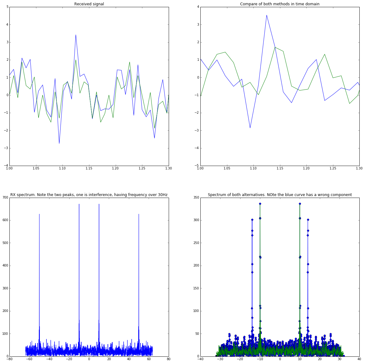
You need to filter first and then downsample. Otherwise, you will run into aliasing problems. I.e. frequencies that are above 30 Hz will create images within your frequencies of interest. You can consider the little script below to compare both methods:
Fs = 128.0
t = np.arange(0, 10, 1/Fs)
signal = np.sin(2*np.pi*10*t) + np.sin(2*np.pi*50*t)
sigma2 = 0.5

rx = signal + np.sqrt(sigma2) * np.random.randn(len(signal))

downsampled = rx[::2]
(b1, a1) = scipy.signal.butter(6, 30/(Fs/4))
down_and_filtered = scipy.signal.lfilter(b1, a1, downsampled)

(b2, a2) = scipy.signal.butter(6, 30/(Fs/2))
filtered_and_down = scipy.signal.lfilter(b2, a2, rx)[::2]
t2 = t[::2]


plt.figure(figsize=(20,20))
plt.subplot(221)
plt.plot(t, rx)
plt.plot(t, signal)
plt.xlim((1, 1.3))
plt.title('Received signal')

plt.subplot(222)
plt.plot(t2, down_and_filtered)
plt.plot(t2, filtered_and_down)
plt.title('Compare of both methods in time domain')
plt.xlim((1,1.3))

f = np.linspace(-Fs/2, Fs/2, 4*len(t))
plt.subplot(223)
plt.plot(f, np.fft.fftshift(abs(np.fft.fft(rx, 4*len(t)))))
plt.title('RX spectrum. Note the two peaks, one is interference, having frequency over 30Hz')

f2 = np.linspace(-Fs/4, Fs/4, 4*len(t2))
plt.subplot(224)
plt.plot(f2, np.fft.fftshift(abs(np.fft.fft(down_and_filtered, 4*len(t2)))), '-o')
plt.plot(f2, np.fft.fftshift(abs(np.fft.fft(filtered_and_down, 4*len(t2)))))
plt.title('Spectrum of both alternatives. NOte the blue curve has a wrong component')

In this script you have a signal that is composed of two sines of frequency 10 and 50Hz plus some noise. In the FFT of the full signal, both spectral lines clearly occur. Now, what you want to have after your signal processing is only one spectral line at 10Hz (because the 50Hz signal should be filtered out). HOwever, if you downsample first, the 50Hz wave is mirrored to $14Hz=64Hz-50Hz$ and cant be filtered out subsequently. Hence, you need to do the filtering before and then downsample your signal.

