7
$\begingroup$

I did search the question database regarding this question, and although one or two questions came close, they didn't really address my specific question.

In adaptive control based on minimizing tracking error (e.g. between plant and model), the designer is free to chose a cost function. More often than not the cost is selected as a function of the squared error.

But I've found in some practical applications that I can achieve a more robust controller by using absolute error. I understand that absolute error provides a more uniform weighting on the size of the error, and I suspect the squared error tends to 'wind-up' the adaptive controller with initially large errors. But I'm not sure how to show this in a generalized way. So I have two questions regarding this:

  1. Is there perhaps a simple analysis that can demonstrate the stability characteristics between absolute and squared error choices in the cost function?

  2. Any references on the matter?

$\endgroup$
7
  • 1
    $\begingroup$ I'm not a controls guy so my opinion matters little. However, I wonder if squared error is typically used because of its obvious connection to least-squares based methods. One nice feature of the squared error cost function versus absolute error: the squared error cost function's derivative with respect to the error is continuous everywhere. The absolute error cost function's derivative is discontinuous near $\text{error} = 0$. I could imagine that this could have implications for stability and/or tracking error. $\endgroup$
    – Jason R
    Commented Sep 8, 2016 at 15:27
  • $\begingroup$ What form does your cost-function have? The standard least-squares cost-function would typically be $J(\theta) = \int_{0}^{t} \left( y(\tau) - \theta(t) u(\tau) \right)^{2} \textrm{d} \tau$. Are you suggesting $J(\theta) = \int_{0}^{t} \left| y(\tau) - \theta(t) u(\tau) \right| \textrm{d} \tau$ instead? $\endgroup$
    – Arnfinn
    Commented Sep 14, 2016 at 10:40
  • $\begingroup$ @Arnfinn my question - more general than specific, but the specific practical work that generated the question is on an application of model reference adaptive control where the plant is considered a scalar and the model is a first order lag. In this application the error was the difference between the output of the closed loop plant using an integrator with adjustable gain, and the model output. The cost I examined was either the square or absolute value of this error. So I guess the answer to your question - yes. But I'm using a gradient (MIT-like) minimization rather than least squares. $\endgroup$
    – docscience
    Commented Sep 14, 2016 at 13:36
  • $\begingroup$ Do you have the book by Ioannou and Sun? amazon.com/Robust-Adaptive-Control-Electrical-Engineering/dp/… $\endgroup$
    – Arnfinn
    Commented Sep 14, 2016 at 23:03
  • $\begingroup$ At any rate, this is a non-linear problem as you probably know, and the general frameworks for stability and convergence analysis would be Lyapunov stability analysis and/or the Grönwall–Bellman lemma... $\endgroup$
    – Arnfinn
    Commented Sep 14, 2016 at 23:06

2 Answers 2

2
$\begingroup$

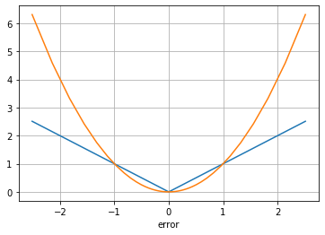
This is an interesting question since both squared error and absolute error are convex functions, so they are both going to give the optimal solution when minimized. My intuition is that the $\ell_2$-norm (sum of squared values of error) converges to zero more quickly than the $\ell_1$-norm (sum of absolute values of error) when the search direction is right. For example, if the error is $\epsilon = y - Ax$. If $y$ is very close to $Ax$ and $0 < |y-Ax| \leq 1$, then $\epsilon^2$ is much smaller than $|\epsilon|$. Similarly, if $|y-Ax| > 1$, then $\epsilon^2 > |\epsilon|$. So the $\ell_2$ norm penalizes large errors more, and small errors less than the $\ell_1$ norm. This can also be understood by looking at the graphs of the two functions when $\epsilon \in \mathbb{R}$.

enter image description here

Of course the continuity of the derivative is another factor. The derivative of the absolute value technically does not exist at the minimum.

$\endgroup$
-1
$\begingroup$

You should use squared error as versus absolute error if you expect to have both positive and negative error values in your population. By squaring the error, only the magnitude of each error value matters (although it is squared). If you want to recover the actual magnitude of error in the population, just take the square root at the end. This value is known as the root mean squared error (RMSE).

If, instead, you were to use absolute error values, the positives and negatives in your population would cancel each other out giving you a false metric.

$\endgroup$
10
  • 1
    $\begingroup$ Hi: They don't cancel each other out using the absolute value just as they don't cancel each other using squaring. There's nothing wrong with the absolute value metric. It's just arises from a different loss function ( loss function is minimized by the median ) and has different statistical properties with respect to robustness, breakdown point, bias, efficiency etc. The squared version is is more popular and can provide an unbiased estimate of the variance, under the normality assumption. But, if this assumption is not true, it is a less robust estimate $\endgroup$
    – mark leeds
    Commented Oct 5, 2018 at 13:09
  • $\begingroup$ @mark_leeds I agree that the absolute error values method does not literally cancel each other out per se, but consider the following special case: error_vals = [ 0, 1, -1, 2, -2, 3, -3, 4, -4] using RMSE, the loss would be Sqrt(50/9) but a calculation using absolute values will result in a loss metric = 0. What am I missing? $\endgroup$ Commented Oct 5, 2018 at 14:04
  • $\begingroup$ Hi: In a rush so just read quickly but where are you getting 0 and sqrt(50/9) from ? Maybe you use it differently, but, AFAIK, using the absolute value in the loss function leads to an more robust estimator such as median, Huber-M location estimator etc so I'm not clear on your numbers. $\endgroup$
    – mark leeds
    Commented Oct 6, 2018 at 16:21
  • $\begingroup$ Hi Mark, Apologies for the typo. Here is how I got the (correct) numbers: RMSE = Sqrt(0+(1^2)+(-1^2)+(2^2)+(-2^2)+(3^2)+(-3^2)+(4^2)+(-4^2))/9. (Note this should have been Sqrt(60/9)). Using absolute values = (0+1+(-1)+2+(-2)+3+(-3)+4+(-4))/9 (Which should be 0/9) $\endgroup$ Commented Oct 8, 2018 at 13:24
  • $\begingroup$ I'm sorry but I don't follow. In the first one, you are calculate the distance between each observation and zero and then squaring that and then adding up over all observations. In the second you are calculating the distance between each observation and zero and then adding up the distances ? This is not what I was referring to as square error estimate versus some more robust estimate. I can't explain it easily here but the squared loss estimator is obtained by mnimizing the expectation of the sum of the squared errors. In this case of the normal distribution, this ends up being the mean. $\endgroup$
    – mark leeds
    Commented Oct 9, 2018 at 15:04

Your Answer

By clicking “Post Your Answer”, you agree to our terms of service and acknowledge you have read our privacy policy.

Not the answer you're looking for? Browse other questions tagged or ask your own question.