Wavelet transform in MATLAB

Question

Suppose I have a wave with $20 \textrm{ kHz}$, $100 \textrm{ kHz}$ and $300 \textrm{ kHz}$. Sampling frequency used is $1000 \textrm{ kHz}$. I apply the discrete wavelet transform on the wave like dwt(wave,'db2'). I will get one level of approximation and detail coefficients. According to the basics, the detail coefficient will have $300\rm k$ component and approximation coefficient will have the $100\rm k$ and $20\rm k$ components

But when I did fft on the output(on approximation and detail), I didn't get what I expected.

• Could anyone post some MATLAB code with which I can verify it?
• And also tell whether I am doing the procedure correctly?
• Also if anyone could explain the practical side of this tool?

Answer 1

What you might be forgetting is that dwt does downsampling. After filtering (low-pass or high-pass), the filtered signal is subsampled. In order to keep the number of samples. So aliasing may occur, depending on the quality of the filters.

And db2 is a quite poor filter. So if you idwt either approx or details, by replacing the other coefficients by zeros, you almost get your coefficients in order: on the top, the original signal, the two low frequencies in the second plot, the high frequencies in the third plot. Of course you have some aliasing, due to the poor resolution.

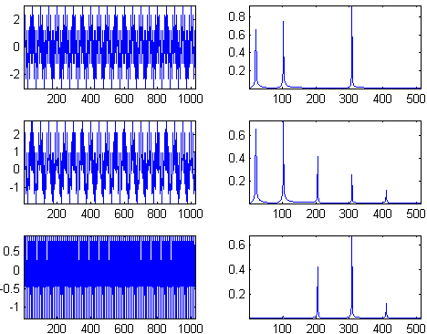
Try the attached code with db24, you will get much less artifact.

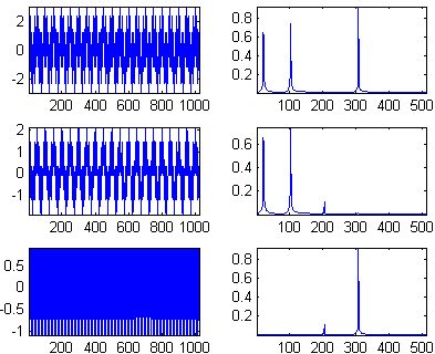
What happens now with the approximation and the details? My interpretation is that the approximation is now sampled at $500$ kHz, and the details too, except that it is now aliased to the base-band:

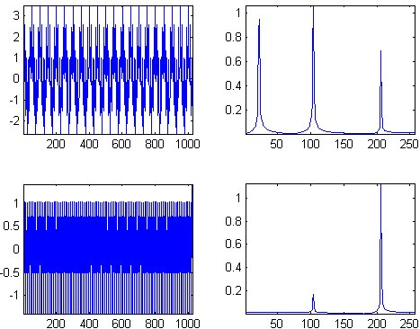
and they need to be unmixed by reciprocal filters of the idwt.

The FFTR.m code should be downloaded.

But why study sines with discrete wavelets?

f = [20/1000  100/1000  300/1000];
nSample = 1024; time = (1:nSample)';
data = cos(2*pi*time*f);
dataSum = sum(data,2);
waveName = 'db2';
[a,d] = dwt(dataSum,waveName);
z = zeros(size(a));

dataSumD = idwt(z,d,waveName);
dataSumA = idwt(a,z,waveName);

timeAD = 1:2*length(a);
timeAD=timeAD(1:2:end);

figure(1)
subplot(3,2,1)
plot(time,dataSum);axis tight
subplot(3,2,2)
plot(FFTR(dataSum));axis tight

subplot(3,2,3)
plot(time,dataSumA);axis tight
subplot(3,2,4)
plot(FFTR(dataSumA));axis tight

subplot(3,2,5)
plot(time,dataSumD);axis tight
subplot(3,2,6)
plot(FFTR(dataSumD));axis tight

figure(2)
subplot(2,2,1)
plot(timeAD,a);axis tight
subplot(2,2,2)
plot(FFTR(a,2));axis tight

subplot(2,2,3)
plot(timeAD,d);axis tight
subplot(2,2,4)
plot(FFTR(d,2));axis tight

So you have the code, I do not know whether you did stuff correctly, and wavelets are quite useful if used widely on signals that are worth it. Sines typically are not on the list.