Help with equations for exponential ADSR envelope

Question

With application code, I have implemented a linear ADSR envelope for shaping the amplitude of an oscillator's output. The parameters for attack, decay and release duration as well as sustain level can be set on the envelope and everything works as expected.

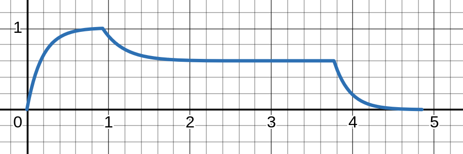
However, I would like to tweak the ramp shapes of the envelope to something that resembles what most synthesizers use for a more natural response: inverse exponential for the attack and exponential for the decay and release. I am having trouble getting my formulas right for calculating the envelope output values for these types of ramp shapes. To calculate the linear ramps, I am using the two-point form, plugging in the start/end $x$/$y$ values which are derived from the attack/decay/sustain/release input parameter values. I cannot seem to work out the correct formula for exponential (standard and inverse) ramps using the same start/end $x$/$y$ point values.

I have saved a Desmos Graphing Calculator session that demonstrates the approach for linear ramps that I described above.

If anyone can help point me in the right direction, it would be much appreciated.

Answer 1

I think that what confuses you is that a decreasing exponential ($e^{-x}$) does never reach 0, so an ADSR generator with truly exponential segments would stay stuck ; because it would never reach the target value. For example, if the generator is at the height of the attack phase (say $y = 1$) and has to land to a sustain value at $y = 0.5$, it can't go there with a true exponential, because the true exponential won't decay to 0.5, it'll only asymptotically go to 0.5!

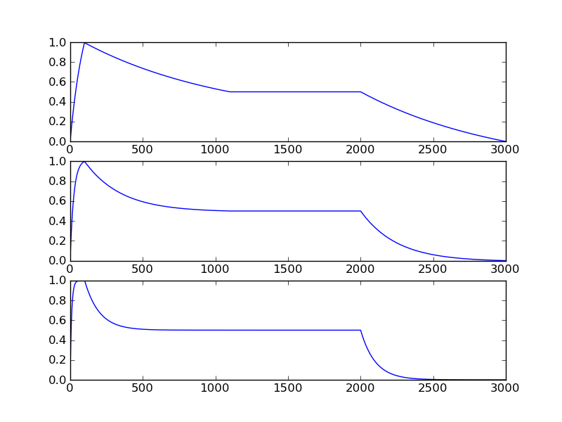
If you look at an analog envelope generator (for example the 7555 based circuit everybody seems to use), you can see that during the attack phase, when the capacitor is charging, it is "aiming higher" than the threshold used to indicate the end of the attack phase. On a (7)555 based circuit powered by +15V, During the attack stage, the capacitor is charged with a +15V step, but the attack stage ends when a threshold of +10V has been reached. This is a design choice, though 2/3 is the "magic number" found in many classic envelope generator, and this might be the one musicians are familiar with.

Thus, the functions you might want to deal with are not exponentials, but shifted/truncated/scales versions of it, and you'll have to make some choices as to how "squashed" you want them to be.

I am curious anyway as to why you are trying to get such formulas - maybe it's because of the limits of the tool you are using for synthesis ; but if you are trying to implement those using a general purpose programming language (C, java, python) with some code running for each sample of the envelope, and a notion of "state", read on... Because it's always easier to express things as "such segment will go from whatever value it has just reached to 0".

My two pieces of advice on implementing envelopes.

The first one is not to try to scale all the slopes/increments so that the envelope exactly reach start and end values. For example you want an envelope that goes from 0.8 to 0.2 in 2 seconds, so you might be tempted to compute an increment of -0.3 / second. Don't do that. Instead, break it down into two steps: getting a ramp that goes from 0 to 1.0 in 2 seconds ; and then applying a linear transform that maps 0 to 0.8 and 1.0 to 0.2. There are two advantages to work this way - the first is that it simplifies any computation you'll have relative to envelope times to a ramp from 0 to 1 ; the second is that if you change the envelope parameters (increments and start/end times) midway everything will remain well-behaved. Good if you're working on a synth, since people will ask to have envelope time parameters as modulation destinations.

The second is to use pre-computed lookup table with envelope shapes. It is computationally lighter, it takes out many dirty details (for example you don't have to bother with an exponential not reaching 0 exactly - truncate it at your whim and rescale it so that it is mapped to [0, 1]), and it's dead easy to provide an option to alter envelope shapes, for each stage.

Here is the pseudo-code for the approach I describe.

render:
  counter += increment[stage]
  if counter > 1.0:
    stage = stage + 1
    start_value = value
    counter = 0
  position = interpolated_lookup(envelope_shape[stage], counter)
  value = start_value + (target_level[stage] - start_value) * position

trigger(state):
  if state = ON:
    stage = ATTACK
    value = 0  # for mono-style envelopes that are reset to 0 on new notes
    counter = 0
  else:
    counter = 0
    stage = RELEASE

initialization:
  target_level[ATTACK] = 1.0
  target_level[RELEASE] = 0.0
  target_level[END_OF_RELEASE] = 0.0
  increment[SUSTAIN] = 0.0
  increment[END_OF_RELEASE] = 0.0

configuration:
  increment[ATTACK] = ...
  increment[DECAY] = ...
  target_level[DECAY] = target_level[SUSTAIN] = ...
  increment[RELEASE] = ...
  envelope_shape[ATTACK] = lookup_table_exponential
  envelope_shape[DECAY] = lookup_table_exponential
  envelope_shape[RELEASE] = lookup_table_exponential

Answer 2

This is a pretty old question, but I just want to highlight a point in the answer from pichenettes:

For example you want an envelope that goes from 0.8 to 0.2 in 2 seconds [...] break it down into two steps: getting a ramp that goes from 0 to 1.0 in 2 seconds ; and then applying a linear transform that maps 0 to 0.8 and 1.0 to 0.2.

This process is sometimes known as "easing," and looks like

$$g\left(x,l,u\right)=f\left(\frac{x-l}{u-l}\right)\left(u-l\right)+l$$

where $l$ and $u$ are the lower and upper bound (possible values being $0$, $1$, and the sustain level) and $f(x)$ is something like $x^n$. Note that you don't need this for the attack phase since it already ranges from $0$ to $1$.

Here is the original Desmos session, updated to use this approach. I used a cubic shape here, but you* could use whatever shape you like, as long as $f(x)$ produces outputs ranging from zero to one given inputs ranging from zero to one.

_{* I guess the OP is probably long gone, but maybe this helps someone else.}

Answer 3

About pichenettes' comment, "During the attack stage, the capacitor is charged with a +15V step, but the attack stage ends when a threshold of +10V has been reached. This is a design choice, though 2/3 is the "magic number" found in many classic envelope generator, and this might be the one musicians are familiar with.":

Any envelope that's shooting for a 15v asymptote with a 10v target is, practically, creating a linear attack. It's just that 15v is the highest asymptote available easily, and it's close enough to linear. That is, there's nothing "magic" about it—they're just going for as linear as they can get.

I don't know how many classic synths use 15v—I'd suspect there's often a diode drop or two. My old Aries modular uses 13v for a 10v envelope, and I just looked up the a Curtis ADSR chip that uses, equivalently, 6.5v for a 5v envelope.

Answer 4

This code should generate similar plots to those of pichenettes:

def ASD_envelope( nSamps, tAttack, tRelease, susPlateau, kA, kS, kD ):
    # number of samples for each stage
    sA = int( nSamps * tAttack )
    sD = int( nSamps * (1.-tRelease) )
    sS = nSamps - sA - sD

    # 0 to 1 over N samples, weighted with w
    def weighted_exp( N, w ):
        t = np.linspace( 0, 1, N )
        E = np.exp( w * t ) - 1
        E /= max(E)
        return E

    A = weighted_exp( sA, kA )
    S = weighted_exp( sS, kS )
    D = weighted_exp( sD, kD )

    A = A[::-1]
    A = 1.-A

    S = S[::-1]
    S *= 1-susPlateau
    S += susPlateau

    D = D[::-1]
    D *= susPlateau

    env = np.concatenate( [A,S,D] )

    # plot
    tEnv = np.linspace( 0, nSamps, len(env) )
    plt.plot( tEnv, env )
    plt.savefig( "OUT/EnvASD.png" )
    plt.close()

    return env

I'm grateful for any improvements, one thing that may be a good idea is allowing the last three parameters (which determine the steepness of each of the three stages) to vary between 0 and 1, where 0.5 would be a straight-line. But I can't see offhand how to do it.

Also I haven't tested thoroughly all usage cases, for example if one stage has zero length.

Answer 5

Here's an extension of P i's post, this is a new account so I can't comment on it. Also I recognize this is a super old thread but I figure ambitious plugin developers like myself are bound to find this in the future.

I added sliders to control the attack, release and sustain, as well as sliders to control the curvature of each stage. I also refactored it by adding negative and zero values for the curvature constants, which affect the graph accordingly.

Pip install matplotlib, ipywidgets and numpy and throw this code into a jupyter notebook and you should be good to go.

import matplotlib.pyplot as plt
import numpy as np
from ipywidgets import interact, widgets

def ASD_envelope( nSamps, tAttack, tRelease, susPlateau, kA, kS, kD ):
    # number of samples for each stage
    sA = int( nSamps * tAttack )
    sD = int( nSamps * (1.-tRelease) )
    sS = nSamps - sA - sD

    # 0 to 1 over N samples, weighted with w
    def weighted_exp( N, w ):
        t = np.linspace( 0, 1, N)
        if w > 0:
            E = np.exp( w * t ) - 1
            E /= max(E)
        elif w == 0:
            return t
        else:
            E = np.exp( w * t ) - 1
            E /= min(E)
        return E

    A = weighted_exp( sA, kA )
    S = weighted_exp( sS, kS )
    D = weighted_exp( sD, kD )

    A = A[::-1]
    A = 1.-A

    S = S[::-1]
    S *= 1-susPlateau
    S += susPlateau

    D = D[::-1]
    D *= susPlateau

    env = np.concatenate( [A,S,D] )

    # plot
    tEnv = np.linspace( 0, nSamps, len(env) )
    plt.plot( tEnv, env )
    plt.savefig( "EnvASD.png" )
    plt.close()

    return env
    

# Create sliders for each function argument
a_slider = widgets.IntSlider(min=0, max=44100, step=1, value=44100)
b_slider = widgets.FloatSlider(min=0, max=1, step=0.1, value=.5)
c_slider = widgets.FloatSlider(min=0, max=1, step=0.1, value=.8)
d_slider = widgets.FloatSlider(min=0, max=1, step=0.1, value=.4)
e_slider = widgets.IntSlider(min=-10, max=10, step=1, value=0)
f_slider = widgets.IntSlider(min=-10, max=10, step=1, value=0)
g_slider = widgets.IntSlider(min=-10, max=10, step=1, value=0)


interact(ASD_envelope, nSamps=a_slider, tAttack=b_slider, tRelease=c_slider, susPlateau=d_slider, kA=e_slider, kS=f_slider, kD=g_slider)

Answer 6

I know this is a 12 year old question, but for anyone else coming along, I think the equation you are looking for is

$$ \frac{2^{cx}-1}{2^c-1} $$

where $x$ is the time variable from 0 to 1 and $c$ is a control variable that determines the shape of the curve, positive or negative.

The output of this function is always $[0,1]$ (while $x$ is $[0,1]$) and the end points stay the same as you vary $c$, so it can easily be stretched and scaled to fit your desired shape.

Here is a Desmos graph where you can play with the control values.

The $2$'s could be $e$ or any other base that is convenient to calculate.

Answer 7

[Repost because the other answer got somehow mangled when it was turned into a comment.]

Comment to @QuinnF's post:

For a parameter $m$ in $[0,1]$ at midtime (as opposed to mid-travel in IEC 60393-1), instead of a parameter $c$, see parameterized potentiometer tapers and Fast Exponential Envelopes:

Fitting of an exponential curve to $f(0)=0, f(1)=1, f(\frac{1}{2})=m$:

$\begin{aligned} f(\varTheta) &= \frac{a^\varTheta-1}{a-1} &\iff f^{-1}(\vartheta) = \log_a(1+\vartheta(a-1)) \\ a &= (1-\frac{1}{m})^2 \end{aligned}$

Linear recurrence with constant coefficients, $F[n] = f(\frac{n}{N})$ and $n=0, 1, \dots, N$:

$F[n] = \begin{cases} 0 &\text{if } n=0 \\ F[n-1] \cdot a^\frac{1}{N} + f(\frac{1}{N}) = F[n+1] \cdot a^\frac{-1}{N} - f(\frac{1}{N}) \cdot a^\frac{-1}{N} &\text{if } 0<n<N \\ 1 &\text{if } n=N \end{cases}$