9
$\begingroup$

Problem.

There is a discrete signal $f[i]$ (example below).
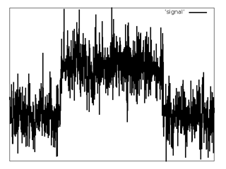
Example of signal
It is known, that $f[i]$ have a form of rectangular pulse with additive white Gaussian noise.

$f[i] = s[i] + n[i]$,
$s[i] = \alpha(\theta[i - i_{1}] - \theta[i - i_{2}]) + c$,
$i_{2} > i_{1}$,
$i_{1} > N$

Where
$\theta[i]$ is a Heaviside step function,
$n[i]$ is an additive white Gaussian noise,
$\alpha$ is a height of rectangular pulse,
$i_{1}$ is an index of the first sample of rectangular pulse,
$i_{2}$ is an index of the last sample of rectangular pulse,
$c$ is constant level of signal,
$N$ is adjustable parameter.

All parameters may have large range of values.
It is required to find value of $(i_{2} - i_{1})$ (duration of rectangular pulse in samples).

Possible solutions.

At the moment, I have tried two ways to solve this problem.

Low pass filter with threshold.

As first attempt, I have used simple scheme with low pass filter and threshold.
1. Apply FIR low pass filter with cutoff frequency equal to $0.05f_{sampling}$.
2. Estimate mean $m$ and dispersion $\sigma^{2}$ of filtered noise from first $N$ samples of the signal.
3. Set threshold $t = m + 3\sigma$.
4. Estimate $i_{1} = \min_{i}(f[i] > t)$.
5. Estimate $i_{2} = \max_{i}(f[i] > t)$.
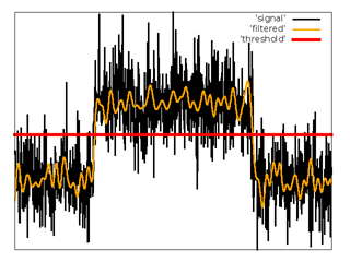
enter image description here

Pros:
1. This algorithm is simple.
2. It is easy to write fast implementation.

Cons:
1. It is hard to estimate efficient value of filter's cutoff frequency. On the one hand low value can corrupt the form of short pulses. On the other hand large value decreases effect from filtration.
2. Algorithm isn't using all information, we have about the signal.

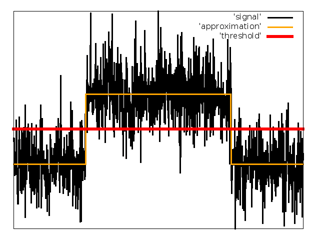
Regression analysis

As the second attempt, I have tried to approximate input sequence of samples with the function $s'[i]$.

$s'[i] = \alpha(\theta'[i - i_{1}] - \theta'[i - i_{2}]) + c$,
$\theta'[i] = \frac{1}{1+e^{-\frac{i}{\beta}}}$, where $\beta$ is a small parameter.

For approximation I have used the method of least squares with gradient descent for minimizing cost function.
1. Set initial values for $\alpha$, $c$, $i_{1}$, $i_{2}$.
2. Perform gradient descent.
3. Set threshold $t = c + 0.5\alpha$.
4. Estimate $i_{1} = \min_{i}(f[i] > t)$.
5. Estimate $i_{2} = \max_{i}(f[i] > t)$.
enter image description here

Pros:
1. This algorithm gives results with good precision.
2. It works for wide range of durations.

Cons:
1. It is very slow.

Question.

After all, I am not satisfied with the precision of the first algorithm and with the speed of the second one. How would you solve this problem?
Is there any classical solution, that I failed to find?
Ideas, links, any feedback will be much appreciated.
Thank you.

$\endgroup$
2
  • $\begingroup$ Do you also need to know the probability that just the random Gaussian noise will cause your algorithm to produce a pulse "duration", especially near the min pulse width and min height you allow? Or is the pulse a-priori known to be present and within allowed parameters? $\endgroup$
    – hotpaw2
    Commented Jan 22, 2015 at 2:50
  • $\begingroup$ @hotpaw2 The pulse is a-priori known to be present and within allowed parameters. If the signal doesn't contain the pulse, then behavior of the algorithm may be undefined. $\endgroup$ Commented Jan 22, 2015 at 9:43

2 Answers 2

6
$\begingroup$

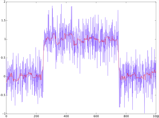
You want a method that removes noise while preserving edges. This cannot be achieved well by linear filtering, as you noticed yourself. I know of two approaches that might work well for your problem. The first is median filtering, where samples inside a window are replaced by their median. The following plot shows the result of median filtering with a window length of 25 samples (in red):

enter image description here

The other, more complex, approach is Total variation denoising, which works very well for piecewise constant signals. There is a very good description of total variation denoising including Matlab code available: link.

$\endgroup$
1
  • $\begingroup$ It was very helpful. And I have had a good time reading the article and playing with the TV denoising. Thank you. $\endgroup$ Commented Jan 23, 2015 at 0:20
2
$\begingroup$

I know this is very old, and @Matt L. long since gave an excellent and informative answer. I had no idea that total variation denoising existed, so I learned something quite useful. Accordingly, I upvoted both the question and answer and want to give a little something, such as it is, back to the site. The basic idea is to use a simple digital version of the old RC LPF and greatly reduce the 'time constant' when a step occurs. Then, after the step, greatly increase the 'time constant'. N.B. The 'time constant' is not really going to be constant, as will be seen below.

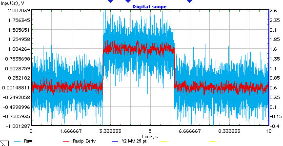
The figure below shows my attempt to replicate the OP's generic noisy rectangular pulse example and how a 'reciprocal derivative' low pass filter (hereafter denoted RD-LPF) performs:

Reciprocal derivative LPF

The RD-LPF is simply $y[i] = Ay[i-1] + (1-A)x[i]$, where $A = exp(-K|y[i-1] - x[i]|)$ and I used $K = 0.2$. The clean rectangular pulse had unit amplitude, started at t = 3 and pulse width was 3. The additive white Gaussian noise had $\mu = 0$ and $\sigma = 0.3$.

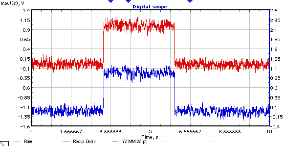
The next figure compares the RD-LPF output (red trace) with (as per Matt L.'s answer) a 25 point moving median filter's output (blue trace):

RD-LPF vs. Mov Med 25 pt

I am not saying I would ever use the RD-LPF for anything serious, but I was curious to see if it would get destroyed in this little comparison. Evidently, that is not the case.

$\endgroup$

Your Answer

By clicking “Post Your Answer”, you agree to our terms of service and acknowledge you have read our privacy policy.

Not the answer you're looking for? Browse other questions tagged or ask your own question.