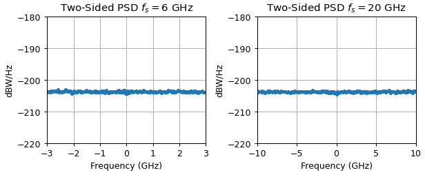
'randn' in Matlab (as well as Octave and Python numpy.random) creates discrete white noise, but it is important to point out that it is not at all "bandlimited". Even if we specify the band edge at Nyquist, the resulting spectrum covers the complete Nyquist bandwidth with a constant power spectral density with no band limiting (the spectrum equally periodically repeats if extended to $\pm \infty$). If we wanted to simulate bandlimited AWGN then we would also need to filter the resulting samples returned by randn. Such filtering is likely not required for the OP's application as the waveform itself is bandlimited, but the added noise need not be (and in many cases to confirm the receiver filtering and performance under noise it is better not - let the receiver do the filtering rather than filter the test signal). Further the following must also be specified which is not clear from the OP:
If the signal to be created is to be complex or real (many baseband simulations are done using complex baseband equivalent signals and would then require noise to be done with a complex white noise source).
If the bandwidth given is "One-Sided" or "Two-Sided". (See this post for further details of these terms and I also provide further explanation in this post later with related plots). I believe from the IR-UWB reference that the passband bandwidth of the signal is 3 GHz (such that if the simulation is done at complex baseband, as I would recommend, then it would have a 3 GHz two-sided bandwidth and be complex).
To complete the answer with a demonstration, I will assume a 3 GHz passband signal, such that the simulation has a 3 GHz Two-Sided bandwidth centered at baseband, as a complex waveform with, importantly, complex AWGN added. We note that the total power of the waveform generated by randn is spread equally across the full Nyquist bandwidth, so the power spectral density (and the resulting total power that falls within the bandwidth) will be set, as I will show, by the standard deviation we use for randn as well as the sample rate.
Thermal noise as given by $kT$ is a flat power spectral density (PSD) that is -203.8 dBW/Hz at room temperature, where dBW is a power ratio in dB relative to 1W, so $10^{-20.38}$ Watts/Hz. $kT$ is also abbreviated $N_o$, but will be $N_o/2$ for Two-Sided passband power spectral densities of real passband signals since half of the noise power is in the positive frequencies and the other half in the negative frequencies. Also for complex (typically baseband) signals, the real or imaginary components alone of a Two-Sided power spectral density will also each be $N_o/2$: If the simulation is a complex baseband simulation, then the total power to be equivalent to thermal noise with no added noise figure would be $N_o$ with $N_o/2$ for the real component and $N_o/2$ for the imaginary.
Typically one wouldn't necessarily need to simulate an accurate thermal noise level for communication system modelling, as simulating signal-noise ratio conditions to test our waveform and receiver processing at sensitivity (minimum received signal level) is often more productive and direct to the issue at hand. With that the approach would be to set the total signal power within its bandwidth, and then the total noise power within that same bandwidth, to arrive at the desired signal-noise ratio. However to show the more complicated case which can then easily simplify to doing an SNR test, I will demonstrate how we could accurately simulate a thermal noise level using the OP's example with an assumed sampling rate of $f_s=6$ GHz and $f_s=20$ GHz. To have units typical of a wireless communication system, I will also assume the waveform is in units of volts, and a resistive impedance of $R=50$ ohms (but other units could be used generally such as $R=1$).
Given the total power of the generated sequence by randn is the variance divided by the resistance when the waveform is in units of volts (regardless of the sampling rate), and it is this power that is spread evenly over the first Nyquist zone, we can determined the standard deviation $\sigma$ (as the square root of the variance) from the desired power spectral density as follows:
$$P_t =\frac{V^2}{R} = \frac{\sigma^2}{R} = kTf_s$$
Where:
$P_t$: Total power in Watts,
$V$: Voltage in Volts,
$R$: Resistance in Ohms,
$k$: Boltzmann's Constant in Joules/Kelvin,
$T$: Temperature (Kelvin),
$kT = N_o$: Power Spectral Density of Thermal Noise in Watts/Hz, $N_o = 10^{-20.38}$ for $T=300$,
$f_s$: Sampling rate in Hz
Thus:
$$\sigma = \sqrt{kTf_sR} \text{ Volts rms}$$
Thus for my examples with $f_s = 6$ GHz and $f_s = 20 $ GHz we have the following standard deviations:
$$\sigma_1 = \sqrt{kT(R) 6e9} = \sqrt{10^{-20.38}(50)6e9} \approx (3.54E-5) \text{ Volts rms}$$
$$\sigma_1 = \sqrt{kT(R) 20e9} = \sqrt{10^{-20.38}(50)20e9} \approx (6.46E-5) \text{ Volts rms}$$
Note for both cases of different sampling rates, the total power due to thermal noise alone at $T=300$ K over the 3GHz of signal bandwidth will be $kTB = -204 \texttt{dBW/Hz} + 10log_{10}(3e9) = -203.8 + 94.8 = -109.0 $ dBW.
The complex baseband AWGN waveform is generated using $\sigma/\sqrt{2}$ for the real component and $\sigma/\sqrt{2}$ for the imaginary component as demonstrated as a column vector created with MATLAB below for nsamps number of samples:
wfm = sigma/sqrt(2) * randn(nsamps, 1) + 1j * sigma/sqrt(2) * randn(nsamps, 1);
The resulting power spectral densities were generated using the welch function on the actual waveforms generated by randn as clarified above using $\sigma_1$ and $\sigma_2$ for each sampling rate, and plotted. We note the strong agreement with the predicted power spectral density given by $kT$ as $-203.8$ dBm/Hz showing the accurate modelling of AWGN (and that it is not at all "bandlimited").

One-Sided vs Two-Sided Spectrums
The spectrums are labeled Two-Sided and are complex, which deserves some additional explanation. A One Sided spectrum for a discrete-time signal, which is only applicable for use with real time domain signals, only extends over the range of DC to Nyquist ($f_s/2$), but is doubled to account for the power from Nyquist to $f_s$, or equivalently the negative frequencies from DC to -$f_s/2$. While a Two-Sided spectrum in comparison extends over the range from DC to the Sampling Rate ($f_s$), or equivalently $\pm f_s/2$. What is more confusing is that for real signals, regardless of "One-Sided" or "Two-Sided" only the positive frequencies (DC to $f_s/2$) are typically plotted (given the redundancy of the negative frequencies since the spectrum is complex conjugate symmetric: the negative frequencies have the same magnitude and negative or conjugate phase of the positive frequencies), such that the Two-Sided PSD will be 3 dB lower than that same plot for the One-Sided PSD.
A practical example where this is actually done in practice from continuous-time systems is oscillator phase noise which is typically given as a Two-Sided spectrum commonly abbreviated as $\mathscr{L}_\phi(f)$, while the equivalent One-Sided power spectral density due to phase fluctuations is indeed 3 dB higher and commonly abbreviated as $S_\phi(f)$.
For complex signals such as those plotted above, the negative and positive frequencies are independent so it makes sense to always show a Two-Sided Spectrum, with the plot extending over $\pm f_s/2$ (or DC to $f_s$) since that would give the complete information.
As far as "bandlimited AWGN" if that was needed for some application, we could proceed to create that from the complex waveforms generated above with randn by passing the waveforms through low pass filters (or bandpass if desired) to achieve the desired spectral shape and bandlimiting.

