2
$\begingroup$

Quick read of my question

The optimum estimator of the mean for N samples of a sampled DC level in the presence of white noise is a block average (an average with all samples given equal weight).

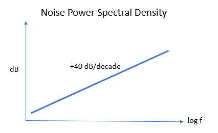
What would be the optimum estimator of the mean for N samples of a sampled DC level in the presence of shaped noise, where the noise is increasing 40 dB/decade?

Noise PSD

More background and motivation for this question:


A delta-sigma A/D converter provides conversion from analog to digital with the benefit of noise-shaping, such that the noise spectral density due to quantization noise is shaped to the higher frequencies (in a typical low-pass delta-sigma converter). I would like to know what the best estimator would be for a DC signal to be estimated with a constraint that the filter impulse response is limited to $N$ samples. "Best" means lowest mean square error. I am assuming the DC input is stationary and the noise in the result is dominated by the shaped quantization noise from the Delta-Sigma (so assume a noise-free DC input).

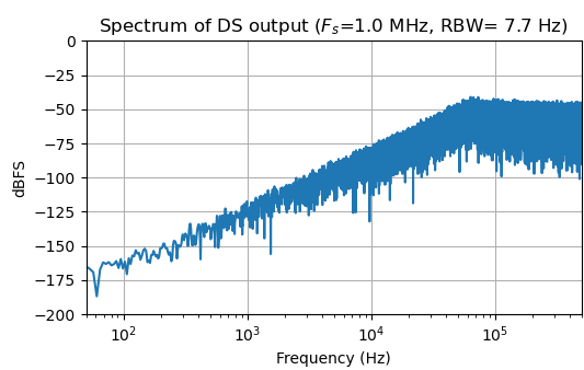
I am also interested in the closest approximation to the Best that can be done with the cascade of moving average filters (such that the cascaded impulse response as the convolution of the individual impulse responses does not exceed $N$). To constrain the solution, assume a 2nd order sigma delta converter which would have a 40 dB/decade high-pass quantization noise shape as depicted in the spectrum plot below.

delta sigma ADC output spectrum

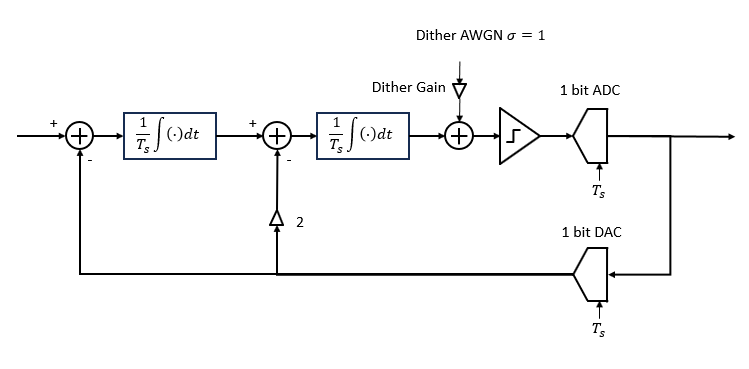
Since some of the answers may assume a dependence on the actual implementation, I provide the implementation details for the assumed Delta-Sigma ADC below (as derived from Slide 16 in Richard Schreier's presentation "Second and Higher-Order Delta-Sigma Modulators MEAD March 2008"). Full scale for the analog input is $\pm 1$, and SNR is maximized at an input level of approximately 50% of full-scale (so my operational full-scale is actually $\pm 0.5$).

Second Order Delta Sigma

Note: Bob made some very helpful comments in his answer, notably that the dither is not necessary if each output as a single average value after N samples is taken on its own (if we are not interested ultimately in the AC performance over multiple successive results). Also the state can be reset in this case after each of the N samples to then be an "Incremental ADC" which is the condition his answer describes, and there is indeed helpful literature on this operation. I will ultimately compare this case (state reset) but want to first evaluate the random start up conditions for purpose of also handling continuous signal conditions (so for this assume the state is not reset every N samples).

I have experimentally come to optimized solutions but am interested if there is a more analytical approach to understand what would optimally be achieved. I understand what is optimum for supressing the Delta-Sigma quantization noise contributions won't be optimum for thermal noise contributions so there will ultimately be a balance with that but wanted to learn from this more specific case narrowed to my opening question (I suspect what is best for shaped noise in general will be best for this mode of operation of the Delta-Sigma due to the randomized output conditions). So far I have found that a Hann Window (which is simply a 0.5-cos() shape over one cycle of the cosine) provides the minimum noise, and I can get close to this by cascading three moving average filters with different lengths (such that the convolution of the three is $N$ samples).

This appears to be a time-bandwidth minimization problem with a fixed duration observation, so I was surprised that the Hann window would be far superior to my typical go-to filters for minimizing time-bandwidth (if you think that is a Gaussian filter, for the case of finite time duration it is not: see DSP.SE 79014). I am curious if the Hann really is Best, or what would be, and then how to make the best approximation to that Best function with moving average filter structures.

$\endgroup$
9
  • $\begingroup$ Oh dear. Not light on content $\endgroup$ Commented May 30 at 21:34
  • $\begingroup$ There is, or used to be, some technology called MASH that was about multistage noise shaping. I don't remember much about it now, but I used to read those papers. Also, unique about 1-bit converters, you have to make a statistical guess about the gain of the converter. For an N-bit flash converter, that gain is the average slope of the staircase function. But when there is a single step, there is no apparent slope to the staircase function. But for the power of the quantization error to be additive to the power of the signal, there is a unique gain. $\endgroup$ Commented May 30 at 21:51
  • $\begingroup$ And remember, even an FIR filter in a feedback loop becomes IIR and you got stability issues to worry about. $\endgroup$ Commented May 30 at 21:58
  • $\begingroup$ Yes I use MASH but that is more about achieving the 2nd order implementation with easier means of maintaining stability and getting closer to full scale, but this is more about the optimum averaging of the result independent of that implementation $\endgroup$ Commented May 30 at 22:32
  • $\begingroup$ So this is FIR after the sigma delta- so no feedback $\endgroup$ Commented May 30 at 22:32

3 Answers 3

2
$\begingroup$

The answer appears to depend on the value of the DC, itself, or rather on the SNR of DC power to noise variance. For a general solution, I would minimize expected estimator variance over the distribution or range of the DC value. Explanation follows below.

Start with the model of a vector of $N$ samples consisting of a DC value plus noise $$ \underline{x} = \alpha \underline{1} + \underline{n} \in \Re^N $$ where $\underline{1}$ is a vector of ones and $\underline{n}$ is a vector of shaped noise with zero mean and covariance $R_{nn}$.

Our objective is to estimate $\hat{\alpha} = \underline{g}^T\underline{x}$ using an MMSE estimation vector $\underline{g}$ to minimize $\mbox{E}[(\hat{\alpha}-\alpha)^2]$. Continuing, \begin{eqnarray} \mbox{E}[(\hat{\alpha}-\alpha)^2]&=&\mbox{E}\left[(\underline{g}^T(\alpha\underline{1}+\underline{n})-\alpha)^2\right]\\ &=&\alpha^2+\underline{g}^T(\alpha^2\underline{1}\;\underline{1}^T +R_{nn})\underline{g} -2\alpha^2\underline{g}^T\underline{1} \end{eqnarray} The MMSE vector that minimizes this estimator variance is then \begin{eqnarray} \underline{g}_{\small MMSE} &=& \alpha^2\left(\alpha^2\underline{1}\;\underline{1}^T+R_{nn}\right)^{-1}\underline{1}\\ &=&\left(\underline{1}\;\underline{1}^T+{1\over \alpha^2}R_{nn} \right)^{-1}\underline{1} \end{eqnarray} Here, the MMSE estimation vector depends on the ratio of $\alpha^2$ to the noise power (diagonal of $R_{nn}$).

Generally, having the estimator of $\alpha$ depend on the value of $\alpha$ is non-ideal, of course. In practice, I would expect to use a reasonable SNR value when determining what to use for $g$ across the expected distribution of $\alpha$ and $R_{nn}$ noise covariance.

$\endgroup$
5
  • $\begingroup$ This is an interesting approach vml- I will try it out later today to verify. Intuitively I feel like it should start with a vector of much longer than N samples such that it is an overdetermined solution. (and still would result in an NxN autocorrelation matrix, but derived from an MxN convolution matrix with M>>N.) This seems similar to what I use for channel estimation described here where t[n] would be the target DC value and r[n] is the DC+noise: dsp.stackexchange.com/questions/31318/… $\endgroup$ Commented Jun 1 at 12:25
  • 1
    $\begingroup$ I'll be interested to hear what you see. I didn't go to the point of creating Rnn and testing. Incidentally, the optimum MMSE estimator of α for white noise is not the simple average with weights of $1/N$, as is shown above with dependence on SNR. For MMSE, we get the equal-weight, $1/N$ average if SNR is infinite. For MVUB estimator, I believe the equal-weight $1/N$ average is the optimum for white noise. I see that you left some ambiguity in your comment about "average with all samples given equal weight" - the term "average" could be taken to mean a biased average that is SNR-dependent. $\endgroup$
    – vml
    Commented Jun 1 at 16:11
  • $\begingroup$ Isn’t it weighted by the SNR per sample (as in maximal ratio combining), such that for white noise and a constant mean, the SNR per sample would be the same and therefore equal weight? It’s not clear to me how we would weigh any samples in the average differently if the SNR is the same per sample (but then with that logic I can’t argue why that changes when I shape the noise so I’m not confident about any of this… yes I’ll provide my results here- thanks for your interest and ideas) $\endgroup$ Commented Jun 1 at 17:11
  • 1
    $\begingroup$ Right, I should clarify on the iid, white noise case. What I mean is that for iid, white noise with finite SNR, the MMSEE uses equal-weight summing but with a scale that is less than $1/N$, producing a biased estimate of $\alpha$ that is closer to zero than a MVUB (min-variance, unbiased) estimate would give on average. Specifically, consider $R_{nn}=\sigma^2I$ in the equation for MMSE $\underline{g}$. In that case, $\underline{g}$ has equal-weight taps but they are smaller than $1/N$. $\endgroup$
    – vml
    Commented Jun 1 at 17:46
  • $\begingroup$ I made an attempt and included it as another answer, along with my code in Python just in case you want to pursue any further. Getting the MMSE to properly converge is not easy so I'm sure there's room for improvement on my attempt using this suggestion of yours. $\endgroup$ Commented Jun 3 at 3:55
2
$\begingroup$

It’s a mistake to consider the spectrum without considering the dynamics of the delta-sigma modulator that produced it. The question you should be trying to answer is the following;

Imagine that you are given a bitstream consisting of N 1-bit modulator outputs, produced by driving the modulator with an unknown DC value X. Now imagine that you have an identical modulator driven with a voltage Xhat. If Xhat=X, then you will get the identical bit stream. However there is some small range delta-X around X that will also give the same bitstream over N samples. Delta-X therefore represents the fundamental limit of precision in estimating X. A good estimate for X is to take the impulse response of the modulator loop filter, truncated to N samples, and then use this as an FIR filter on the modulator bitstream (or if you just want a single estimate, use the dot product). I have a no-math explanation of this that I used to use in a course I taught 20 years ago; if people are interested I could probably dig it up.
Note also that this is highly related to the so-called “incremental a/d converter”, and a search on this topic will yield many results.
For example; https://ieeexplore.ieee.org/document/9152080

$\endgroup$
9
  • $\begingroup$ Hi Bob-Thanks for this. This sounds like a "matched filter" approach which makes sense as an optimum solution. Although I would have assumed it would be impulse response for the closed loop Noise Transfer Function, not the open loop Loop Filter, also my "loop filter" for the 2nd order implementation is a bit more complicated as it is two integrators in cascade. I'll add the block diagram to my question to be clear on the implementation in case you can specify a specific filter I can try for this case. $\endgroup$ Commented Jun 2 at 14:35
  • $\begingroup$ (ultimately I suspect the solution can be driven from the PSD alone, and should be reasonably close, that PSD is directly related to the Noise Transfer Function so we may see that it converges to the same answer- also I am using white noise dithering to randomize any bit patterns that would be evidenced in spurs) $\endgroup$ Commented Jun 2 at 14:37
  • $\begingroup$ Dan, if you’re using dither then things are different. In a traditional incremental converter, you run the the modulator for N samples, then perform a weighted summation on the bits, and then you reset the modulator and start again. So there’s no concept of idle tones. If you’re working in an application where you are producing a continuous bitstream and looking for optimal AC performance, then dither makes sense, and the technique of incremental A/D converters does not apply (although if you know the dither sequence you might be able to subtract it later) $\endgroup$
    – Bob
    Commented Jun 2 at 18:09
  • $\begingroup$ right. Hopefully you see the focus of my question. The cascade of moving averages (higher order CIC) is the typical approach for this, and results in a very good estimate. I just got in the weeds of technical interest in what would be optimum for the given noise spectrum, finding that I could get there by trial and error but couldn't quite see through the analytical approach to what would minimize the noise - what vml suggests sounds promising and I am going to try that and will report my results here- if you have a particular filter based on your "matched filter" approach... $\endgroup$ Commented Jun 2 at 18:23
  • 1
    $\begingroup$ Dan, I found my no-math slides, see the following ppt, slides 32-36. dropbox.com/scl/fi/13e8fnrpcnwy33ty6fqq4/… $\endgroup$
    – Bob
    Commented Jun 2 at 23:02
1
$\begingroup$

I will provide the details of my own evaluation as an answer, including that of other answers provided. If anyone can provide a filter solution that out-performs the filter using the Hann window as coefficients, I can add it to the test cases below and will select that as the right answer (or if someone can provide an analytical explanation as to why Hann would be optimum, if it was).

Test Conditions: 2nd order Delta Sigma Modulator with input = 0.5 (Full scale= +/-1), Maximum Averaging Window = 512 samples. Sigma Delta is not reset after N samples (This is not an "incremental ADC" in that the Sigma Delta is never reset, so takes further advantage of randomization from multiple results of N sample blocks for AC performance, however I will test the incremental case as well to see if the solution holds up either way).

Python code to create test waveform:

import numpy as np    # provides fastest dither generator
def DsADC(m=1, dither_gain=0, debug=False, init =(0,0,0,0,0,0)):
    '''
    2nd order Delta Sigma ADC as a coroutine generator
    use: 
    ds = DsADC()
    ds.send(None)   # prime
    output_sample = ds.send(input_sample)    

    Dan Boschen 1/15/2023

    Initialization Parameters
    ----------
    m: oversampling factor to model continuous time integrators using accumulators.
    dither_gain: multiplication factor to add random noise dither
    debug: will return all internal states when True (defaults to False)
        states: out, delta1, sum1, sum2, fb 
    init: setting for initial states (defaults to all zeros)
    
    Returns
    -------

    ds_gen: generator iterator
        Generator returns out: digital values vs time as ints 0 or 1

    Note: this is a floating point implementation so will 
    ultimately overflow for very long runs without resetting.
    '''

    # initialization
    count = 0
    out, delta1, delta2, sum1, sum2, fb  = init
    full_scale = 1
    dither = 0
    # run ADC
    while True:

       # compute next state (clock update)
        sum1d = sum1
        sum2d = sum2
        
        if count % m == 0:
            # get next input, provide last output
            if debug:
                sample = yield out, delta1, delta2, sum1, sum2, fb
            else:
                sample = yield out
            if dither_gain:
                dither = np.random.randn()
            # ADC update: update out and fb
            out = 0 if sum2 + dither_gain * dither < 0 else 1
            fb = -full_scale if out == 0 else full_scale
            delta1 = sample - fb
            delta2 = sum1 - 2 * fb
               
        sum1 = (sum1d + delta1/m)
        sum2 = (sum2d + delta2/m)
        count +=1

Using the above code, samples of the waveform are created as follows:

# Create DC Test Signal:
nsamps = 2**18   # total number of samples
waveform = 0.5 * np.ones(nsamps)
ds1 = DsADC(m = 10, dither_gain=1.5, debug=False)
next(ds1) # prime coroutine
# scaled output for average in range +/-1 to match input:
result = 2* np.array([ds1.send(i) for i in waveform]) - 1

And the SNR result for any filter with coefficients given as coef are tested with:

import scipy.signal as sig
def eval_coef(coef, result):
    filt_out = sig.lfilter(coef, np.sum(coef), result)[len(coef):]
    return 20*np.log10(np.abs(np.mean(filt_out))/np.std(filt_out))

Test Results (All filters total length = 512)

Hann:


hann = sig.windows.hann(filt_dur)
print(f"Hann Filter: {eval_coef(hann, result):0.2f} dB")

Hann Filter: 86.3 dB

Simple cascade of 1/3 length moving avg filters:


mavg = np.ones(int(filt_dur/3)+1) 
mavg2 = np.ones(int(filt_dur/3)+2)
coef = np.convolve(mavg, mavg)
coef = np.convolve(mavg2, coef)
print(f"Mavg x3 Filter: {eval_coef(coef, result):0.2f} dB")

MAVG171+MAVG171+MAVG172: 83.7 dB

Cascade of optimized length moving avg filters:


Instead of 3 moving averages in cascade all equal in length (which is approximately 1/3 of the total filter span), I tried modifying the lengths to take advantage of the smaller main-lobe in frequency of a longer moving average, while still getting the 3rd order roll-off of the three moving averages at higher frequency offsets. Experimentally I came up with a 257 length moving average, cascaded with a 171 length moving average and an 86 length moving average.


# 3 moving avg filters with different lengths
mavg = np.ones(int(filt_dur/2)+1) 
mavg2 = np.ones(int(filt_dur/3)+1)
mavg3 = np.ones(int(filt_dur/6)+1)
coef = np.convolve(mavg2, mavg3)
coef = np.convolve(mavg, coef)
print(f"MAVG257+MAVG171+MAVG86: {eval_coef(coef, result):0.2f} dB")

MAVG257+MAVG171+MAVG86: 86.0 dB

VML Least Squares:


I attempted VML's least squares solution as follows:

import scipy.linalg as la
x = result[:filt_dur]    
alpha = 0.5      # target DC value
n = x - alpha    # noise vector

def convmtx(h,n):
    # creates the convolution (Toeplitz) matrix
    # h is input array, 
    # n is length of array to convolve 
    return la.toeplitz(np.hstack([h, np.zeros(n-1)]), np.hstack([h[0], np.zeros(n-1)]))

A = convmtx(n, filt_dur)
R = np.dot(np.conj(A).T, A)    # autocorrelation matrix
coeff = la.solve((np.ones((filt_dur, filt_dur)) + R / alpha**2), np.ones(filt_dur))

This resulted in a post filtered SNR of 58.64 dB. I tried increasing the length of x so that more of the noise is included in the solution (leading to an overdetermined system of equations as desired for the least squares solution), but I couldn't increase the length more than 2x without it crashing my analysis. By changing the second line to be x = result[:2 * filt_dur] (twice the number of coefficients), the solution improves to 64.2 dB. I assume if this could be implemented more efficiently, and with a starting length > 20x the desired number of coefficients, that it may provide an optimized result.

A plot of the resulting coefficients for the VML 2x case, and the hann window and optimized 3x moving average is below:
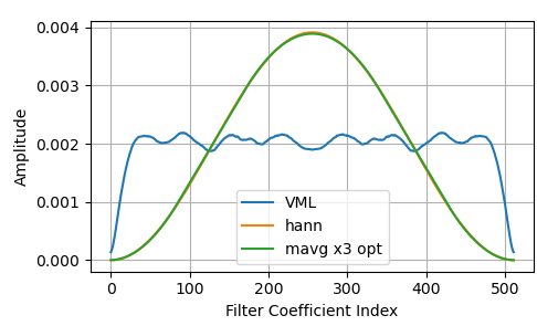
resulting coefficients

Bob's Matched Filter:


I attempted Bob's approach of time-reversing the loop filter response as follows:

Create filter coefficients as the truncated and time reversed impulse response of the loop filter given by $H(z) = \frac{z^{-2}-2z^{-1}}{(1-z^{-1})^2}$, or simply the cascade of two accumulators (I tried it both ways shown below and confirm that both produce the same result):

impulse = np.ones(filt_dur)
impulse[0] = 1
imp_resp = sig.lfilter([1, -2, 0], [1, -2, 1], impulse)
coef = imp_resp[::-1]
coef = coef / np.sum(coef)


coef2 = np.cumsum(np.ones(int(filt_dur)))
coef2 = np.cumsum(coef2)
coef2 = coef2 + 2 * np.cumsum(np.ones(int(filt_dur)))
coef2 = coef2[::-1]
coef2 = coef2 / np.sum(coef2)

This resulted in a post filtered SNR of 38.0 dB. A plot of the resulting coefficients is shown below:
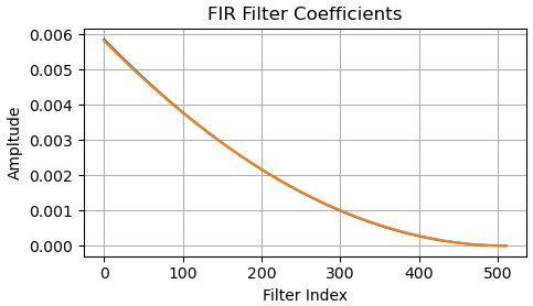
Coeff for double summation

I believe the remaining issue here is that the truncation of what should be a 2nd order response results in a filter that only has a first order roll-off (the 2nd order response convolves in frequency with a Sinc resulting in the first order response). I tried multiplying the impulse response with various windows including one-sided and early-weighted windows, which corrected the roll-off but the best I could get was multiplying with the symmetric Hann, and for that I got an SNR of 81.7 dB, which is worst than just using the Hann directly).
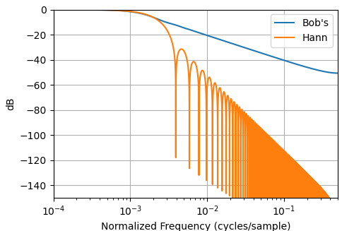
Frequency Response comparison


Note I also characterized my Delta-Sigma DAC model by evaluating the SNR for 500 different DC levels swept over a logarithmic range from $10^{-3}$ to $10^{-0.1}$ to confirm for lower levels the output changes dB for dB with the input level, and to determine where the optimized full-scale operation would be:
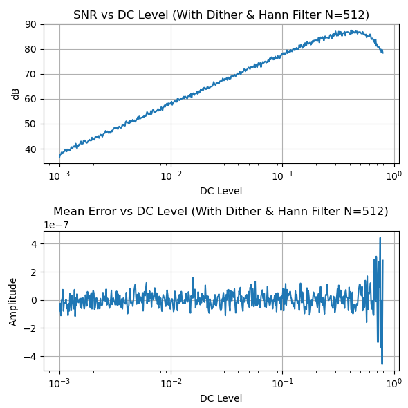
SNR vs DC Level, with Dither

I think I initially misinterpreted a comment Bob made below his answer about dither, and that he was actually suggesting dither is not necessary for my use case (if I am only interested in the DC value at the end of each epoch). For comparison, I ran the above test with no dither ( although for this test I did not reset the system for subsequent epochs, nor does it demonstrate ac performance):
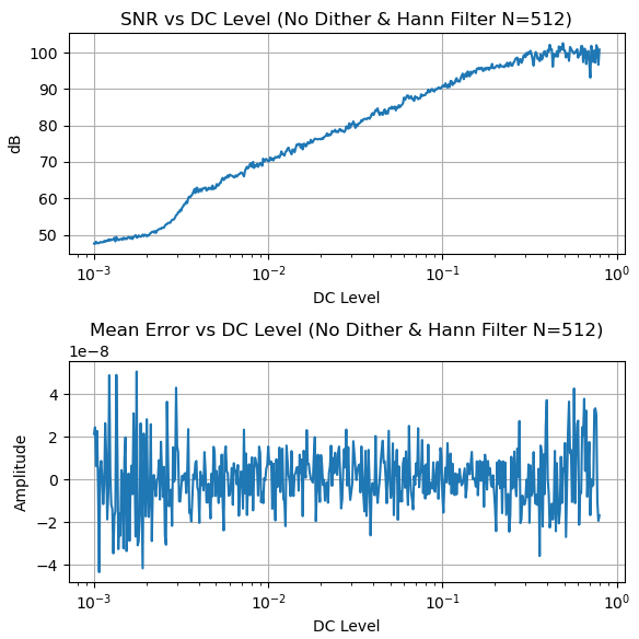
SNR vs DC Level, no Dither

After repeating the comparisons with an input level of 0.612 and no dither, filter length= 512, the table below summarizes all results:

Filter (N=512) Dither, input = 0.5 No Dither, input = 0.612
Hann 86.3 dB 99.5 dB
MAVG171+MAVG171+MAVG172 83.7 dB 98.2 dB
MAVG257+MAVG171+MAVG86 86.0 dB 99.0 dB
VML Least Squares* 64.2 dB **
Bob's Matched Filter*** 38.0 dB 44.1 dB

*$\space$My attempt thus far at VML's suggestion; I suspect this can be improved and not a limitation of the suggestion
** Did not properly converge (as limited by my implementation of the suggestion)
*** As I interpreted his description. Windowing the coefficients improves this, but not as good as other results shown.

$\endgroup$

Your Answer

By clicking “Post Your Answer”, you agree to our terms of service and acknowledge you have read our privacy policy.

Not the answer you're looking for? Browse other questions tagged or ask your own question.