Even after applying a low pass filter, why is there a DC offset?

Question

I need to smooth some data segments and one of the techniques I am experimenting is a low-pass filter. So I designed a low-pass filter in matlab and applied it to my signals. Here is what happened with two of them.

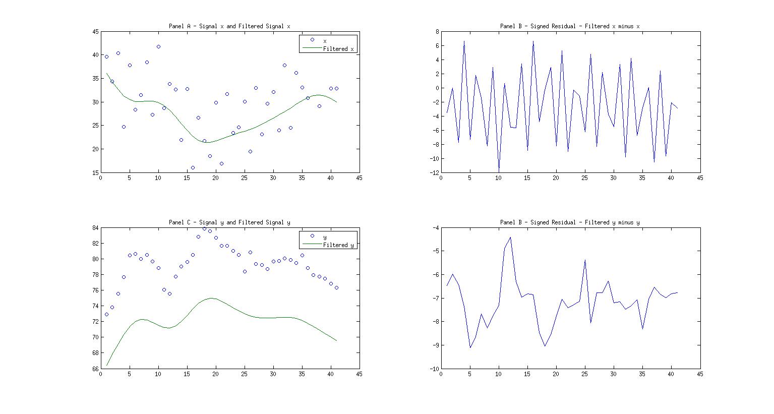
Panel A is one of the data segments plotted with its filtered signal. It looks good. This is what I expect and Panel B is its signed residual which is the filtered signal minus the original signal. I see there is no DC offset and no linear trend so I am happy.

Panel C is another data segment plotted with its filtered result and there is an obvious offset between the two. The filtered signal "doesn't run through" the signal like how I think it should. Panel D is its residual and we confirm that the mean is not zero. And sometimes (not shown here) I see a linear trend as well in the residual.

So my question is what is going on here? How should one interpret this? I am using low-pass filtering so the DC component should be included so the mean of the residual should be close to zero. Does this say something about the power at high frequencies like is there "too much" power at higher frequencies? Something with leakage or something like power leaking from the zero channel to other neighboring frequencies? Maybe I did something wrong? Is there anyway to fix this? I need to be sure that all of the residuals are like Panel B with no linear trends and the mean being around zero.

The bigger focus is to look at both the smoothed signal (the low-pass filtered signal) AND the residual with the emphasis being on the residual. If this can be fixed then good otherwise I am thinking after filtering like this, then subtracting a least squares fit straight line from the residual. Then adding the signed residual to the original signal to get the smoothed-version that goes "through" the signal.

Yep, I know guys that generally it isn't a good idea to low-pass and subtract. But long story and I have no choice. As you can see in the code, the data segments all have length 41 with 30 seconds cadence so the frequency step size is 0.000813 which is of course also the first bin after the zero channel. So what I am trying to do is to get rid of the power in the zero channel and then look at all other (higher) frequency bins so in other words, detrending (hence my cutoff frequency at 9mHz). The problem is that I need a smoothed version of the signal as well as the detrended signal. So as far as I can tell, either low pass and then subtract...OR...high pass and then add.

Thanks everyone.

Here is my code

% Filter Design
Fpass = 1e-09;   % Passband Frequency
Fstop = 0.009;   % Stopband Frequency
Apass = 1;       % Passband Ripple (dB)
Astop = 60;      % Stopband Attenuation (dB)
Fs    = 1/30;    % Sampling Frequency
h = fdesign.lowpass('fp,fst,ap,ast', Fpass, Fstop, Apass, Astop, Fs);
Hd = design(h, 'equiripple', ...
        'MinOrder', 'any', ...
        'StopbandShape', 'flat');
xavg = filtfilt(Hd.numerator,1,x);
yavg = filtfilt(Hd.numerator,1,y);
xdelta = xavg - x;
ydelta = yavg - y;

t=1:41;

figure
subplot(2,2,1)
plot(t,x,'o',t,xavg)
legend('x','Filtered x')
title('Panel A - Signal x and Filtered Signal x')
subplot(2,2,3)
plot(t,y,'o',t,yavg)
legend('y','Filtered y')
title('Panel C - Signal y and Filtered Signal y')

subplot(2,2,2)
plot(t,xdelta)
title('Panel B - Signed Residual - Filtered x minus x')
subplot(2,2,4)
plot(t,ydelta)
title('Panel B - Signed Residual - Filtered y minus y')

---

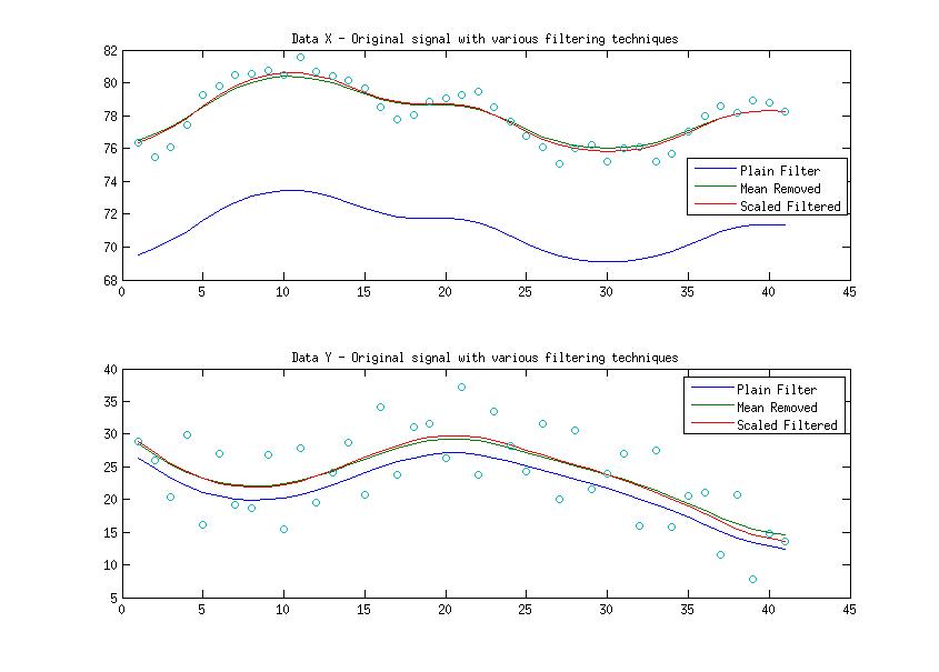
Edit: I didn't see the comments before. I just saw them right now and checked out what geometrikal pointed out. And here is the pic different data sets but same idea. I couldn't find the original numbers I used so just took another set of numbers. So here I am only plotting two signals, no residuals. Call the top X which gives a bigger offset and the bottom Y. So for both of the signals, I plot the signals with results of the various filtering methods. Here is the code to show what I am doing.

% Just normal filtering
xfilt = filtfilt(Hd.numerator,1,x);
yfilt = filtfilt(Hd.numerator,1,y);

% Filtering by subtracting the mean and then adding it
xfiltmean = filtfilt(Hd.numerator,1,x-mean(x))+mean(x);
yfiltmean = filtfilt(Hd.numerator,1,y-mean(y))+mean(y);

% The scaled filter
sc = mean(filtfilt(Hd.numerator,1,ones(1,41)));
xfiltsc = xfilt/sc;
yfiltsc = yfilt/sc;

and yep the filter doesn't sum to one as the picture clearly shows. sum(Hd.numerator)=0.9546 so which one of the two is the problem is this? What does this mean? Is it the zeropadding or this scaling thing? Because applying both of these fixes individually seems to work or at least they give roughly the same answers. Both of them together like this

(filtfilt(Hd.numerator,1,x-mean(x))+mean(x))/sc;

won't work because now the filtered signal will clearly be too large (and verified this with my data). And the magnitude of the data doesn't seem to matter even if I do

x = x+1000;

I get the same results. Both filters are almost identical. So which fix should I apply? Removing the mean or scaling?

Thanks guys for all your help.

Answer 1

It could be a few things.

Zero padding of the input signal:

Some filtering operations pad the end of the signal with zeros before convolving it with the filter kernel. I don't think filtfilt does this though.

Filter doesn't sum to 1:

Lets say you had a discrete signal that was all 1's. The low pass filtering should also return all 1's. Because you are operating on discrete signals, even if the filter is designed properly the errors that come in through discretisation can cause the filter to give a different value. For example, compare the discrete Gaussian kernel to the sampled Gaussian kernel below (image taken from wikipedia, more info at http://en.wikipedia.org/wiki/Sampled_Gaussian_kernel). I think this is the most likely explanation. You could scale your filter output as a crude fix.

The Gaussian kernel is often used for low-pass smoothing because it generates a scale-space. In practice this means that smoothing does not generate any new features in the signal, and that more smoothed signals will always have the same or less detail as less smoothed signals. I would try that if you haven't already.

Answer 2

The DC offset is just the average of all your samples. You should calculate that first, subtract it, then run your filter.

I think what is happening here is that your data is getting padded with zeros on the left and right, so you are actually averaging your real data with a bunch of extra zeros. (I don't know matlab, so I may be very wrong about this.) So the DC value you are getting right now is way off (low because your data is all large and positive.)