FIR filter design with nonlinear phase from measured amplitude and phase responses

Question

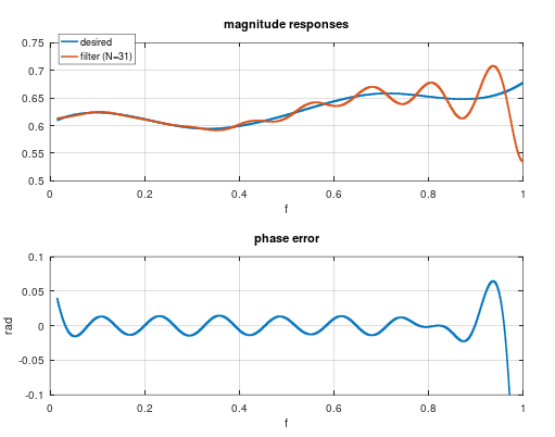
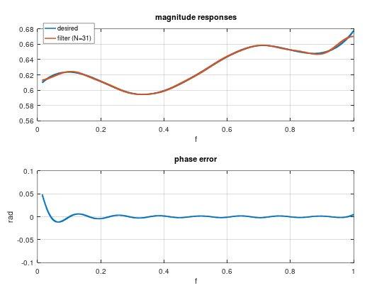
I am having trouble when design FIR filter fitting to the complex data (i.e., amplitude and phase responses from measurements). I did try to use Matt. L's lslevin method here since this method is to deal with arbitrary prescribed amplitude and phase. However, it seems that I cannot get the appropriate real time-domain coefficients. You may run the Matlab script to check the results.

The issues I did encounter were that the amplitude and phase estimated from lslevin result present huge errors compared to the original measured data.
I have also checked with various design method listed in Matt. L. PhD thesis, but I still have not found a solution.

It would be great help if you have any suggestions or solutions.
Thank you very much.

Matlab script for illustration:

% FIR filter design using LS method with arbitrary amp. & phase resp.
% (nonlinear phase)
clc;close all;clear all

%% setups & measurement results
fs = 16e9;
fn = 31/4096*fs:125e6:2047/4096*fs;
f_norm = 2*pi*fn/fs;
fn_intp = linspace(f_norm(1),f_norm(end),512);
amp0 = [0.6100 0.6082 0.5949 0.6309 0.6582 0.6482 0.6775];
phs0 = [0.0465 0.0465 0.2740 0.8148 1.0403 1.8896 2.5158];
f_meas = [f_norm(1) f_norm(14) f_norm(20) f_norm(35) f_norm(45) f_norm(55) f_norm(end)];

% interpolation to have dense data
amp = interp1(f_meas,amp0,fn_intp,'spline');
phs = interp1(f_meas,phs0,fn_intp,'spline');
figure;plot(fn_intp,amp);figure;plot(fn_intp,phs);

%% Test with Matt. L.'s alg.
D = amp.*exp(1j*phs);% desired response
W = [ones(1,32) ones(1,448) ones(1,32)];% weighted 
tap_num = 11;
h = lslevin(tap_num,fn_intp,D,W); % please download the lslevin function
figure;stem(h,'linewidth',2);grid on;xlabel('Index');ylabel('Amp.')

% plot to check
[A,F] = freqz(h,1,512);
figure;plot(fn_intp,amp);grid on
hold on;plot(F,abs(A));xlabel('Norm freq. (rad./sample)');ylabel('Amp.')
legend('Original','LS results')
figure;plot(fn_intp,phs);grid on
hold on;plot(F,angle(A));xlabel('Norm freq. (rad./sample)');ylabel('rad.')
legend('Original','LS results')

Answer 1

The algorithm gives you the best least squares approximation possible for a causal filter with the specified filter order and the given desired frequency response. The problem with your specification is the desired phase response. It corresponds to a negative group delay almost throughout the entire band. Apart from that, a real-valued filter must have a phase of zero or $\pm\pi$ at DC and at Nyquist, which the given phase response doesn't satisfy either.

If you really need to approximate the given phase response, the only option for obtaining a reasonable approximation with a causal filter is to add a linear phase to the desired phase. This just means that the filter adds some delay apart from approximating the desired phase response. This is usually no problem, and in this case there's no other option anyway.

I tried this by adding the following lines to your code (after the interpolation of the data):

del = 15;
phs = phs - fn_intp * del;

This adds a linear phase for a specified delay del. I also increased the number of taps to $31$.

tap_num = 31;

Note that the extra delay del should be adapted to the number of taps, i.e., if you want to increase the number of taps you should also increase the delay.

The figures below shows the approximation after these changes. The top figure shows the desired and actual magnitude responses, and the bottom plot shows the phase approximation error. The result is still not great because the phase at Nyquist is not what a real-valued filter can realize.

The result can be further improved by changing the phase specification at Nyquist such that the phase remains smooth but that its value at Nyquist equals an integer multiple of $\pi$, which is what a real-valued filter can satisfy. The phase value closest to the one specified at Nyquist is $\pi$. Changing the definition of phs0 to

phs0 = [0.0465 0.0465 0.2740 0.8148 1.0403 1.8896 pi];

changes the result significantly. With del=15 and tap_num=31 the design results are shown in the figure below: