5
$\begingroup$

I have never fully been able to wrap my head around Fourier transforms, so I apologize if what I am trying to do is trivial or violates basic theory in some way.

What I have is a "made up" frequency spectrum (well, it comes from somewhere but not relevant for my problem). The spectrum has the form:

$$|G(\omega)| = \frac{a}{\sqrt{b\omega }}$$

where $a$ and $b$ are arbitrary (real) constants for my particular application. Note that I only show the spectrum but the real complex-valued Fourier spectrum would be: $$G(\omega) = \frac{a}{\sqrt{b\omega }}e^{i\phi(\omega )}$$

For my purposes, $\phi(\omega)$ can be anything and is not physically constrained. As a starting point I've just set $\phi(\omega)=0$ so that the spectrum is real-valued. Sampling rate (or frequency spacing) can be arbitrary as can the length of signal.

What I want to do is find a time series, $g(t)$ that is the inverse Fourier transform of $G(\omega)$.

What's the easiest way to do this?

Thus far, I've done it an exceedingly "dumb" way that probably makes many specialists in time series processing cringe. I've basically just digitized the frequency spectrum like a comb filter and then calculated the sinusoids at each spike in the comb and then added them together. Basically treating each individual digitized frequency as a delta spike (implemented in MATLAB below), using the most basic defintion of the Fourier transform:

$$ g(t) = \int_{-\infty}^{\infty} A(\omega)e^{i2\pi\omega t} d\omega$$ The resulting time series I get actually kind of looks "okay" on first glance. However, if I try to perform a standard MATLAB fft of this time series, it returns complete garbage (see figures below)

Code:

N = 1000; %number of discrete frequencies to digitize the continuous spectrum
a = 1.2566; %constant
b = 0.00078956; %constant

w = 10.^linspace(0,-4,N); %get logarithmically spaced frequencies omega

%The spectrum
G = a./sqrt(b*w);


M = 100000; %length of time series
fs = 1; %assuming a 1 Hz sample rate

t = linspace(0,fs*M,M)';

%the time series is computed as a "dumb" Fourier transform which assumes
%that each discrete frequency is a delta spike respresenting a time-domain
%sinusoid. Just sum it all together:
g = sum(G.*exp(1i*2*pi*w.*t),2); 


%Now perform fft on the time series you just made
pad = 10000;
xt = cat(1,ones(pad,1).*g(1),g,ones(pad,1).*g(end)); %add some padding cells to the time series
X = fft(xt); 

%Calculate frequency bins
df = fs/length(xt);
fAxis = (0:df:(fs-df)) - (fs-mod(M,2)*df)/2;

%Plotting
subplot(2,1,1) %Plot spectrum
loglog(w,G,'*r'); hold on; grid on
loglog(fAxis,abs(X),'-k'); 
xlabel('Frequency (Hz)');
ylabel('G(\omega)')
set(gca,'FontSize',14)
title('Spectrum G(\omega)')
legend('"True" Spectrum','FFT of Time Series')

subplot(2,1,2); %Plot time series
plot(t/3600,real(g)); hold on;
xlabel('Time (hours)')
ylabel('g(t)'); grid on
set(gca,'FontSize',14)
title('Inverse "Fourier Transform" of Spectrum')

Result:

enter image description here

Any help is appreciated!

$\endgroup$
3
  • $\begingroup$ Don't confuse FT with DFT. Work purely with FT, and as long as the sampling rate is sufficiently great and code matches math, stuff should work out. Ignore advice that says "finite in time requires infinite sampling rate". $\endgroup$ Commented Jun 1, 2023 at 21:43
  • 1
    $\begingroup$ This is only marginally related, but what you're trying to create here is a "pinking filter". This is a filter in which flat white noise (which is what comes out of a good random number generator) goes in and pink noise comes out. A simple and crude approximation using a 3rd-order IIR filter can hit this within ±0.3 dB can also be done. $\endgroup$ Commented Jun 11, 2023 at 19:23
  • $\begingroup$ @robertbristow-johnson That's a really good and practical solution. When/if I have some more time, I'd like to update my comparison chart showing the error vs different methods that is at the end of my answer to include that. $\endgroup$ Commented Jun 13, 2023 at 4:20

3 Answers 3

5
$\begingroup$

Bottom Line

  • OP's approach is closest to the "Frequency Sampling Method"
  • Use a linear frequency grid, not logarithmic.
  • Populate the spectrum on both the positive an negative frequency axis, with complex conjugate symmetry for real time samples.
  • (As MattL pointed out): bound the DC bin to a finite value.

The OP's used logarithmically spaced positive axis only frequencies but proceeded with what is equivalent to a Discrete Fourier Series reconstruction where linearly spaced frequencies should be used. Using linear spaced frequencies that include the positive and negative frequencies, and using the inverse FFT directly to estimate the time domain response results in the "Frequency Sampling" method. The plot below shows the achievable result of the recreated spectrum using 1001 samples as the OP had done. Increasing the number of samples extends the accuracy to even lower frequencies.

spectrum

The remaining details in this post should clear up any disconnects with the OP's initial intuition with the approach that was attempted.

MORE DETAILS

The main points of this post, including what was wrong with the OP's initial attempt is concluded above. The remaining part of this post details the deeper considerations needed to do the Frequency Sampling Method properly for any generic spectrum (real or complex), and then as an interesting study I included a direct comparison to the result for the Windowing Method that MattL derived in his answer (initially I expected the Frequency Sampling solution using the same number of samples to be worst without increasing the density of samples in frequency and wanted to demonstrate that, but that didn't turn out to be the case). That later section also summarizes the differences and approach of the two methods.

The Frequency Sampling method is simple and quite effective if you are able to sample the frequency over the spectrum of interest with fine enough spacing to avoid time domain aliasing distortion. To proceed, sample the desired spectrum using both its magnitude and phase, and then use an inverse FFT calculation to determine the time domain samples. The finer the spacing in frequency that is used, the longer the resulting time domain response will be, which will further reduce deleterious time-domain aliasing effects. This resulting time response can be truncated to a smaller duration, and then this result windowed to reduce the time-domain truncation effects. Without such windowing the time-domain truncation will result in ripples in the frequency response. Extending the sampling rate higher (most simply by zero-padding the target spectrum) is also an effective approach to interpolate more samples in the resulting time domain response if needed.

There are some details that are important to be aware of:

Detail 1 With using the inverse FFT directly, the sampled frequency domain must extend from DC to 1 sample less than what will be the sampling rate for the resulting time domain signal. This is to properly fill the values that essentially are the FFT result: $N$ samples in time are $N$ samples in frequency, the first FFT bin with $k=0$ is at "DC" and the last FFT bin with $k=N-1$ is at the frequency that is nearly the sampling rate (if there was one more bin at $k=N$, it would be at the sampling rate). The upper half of this spectrum is equally the "negative frequencies" due to periodicity of the FFT. Assuming a real time domain response, each negative frequency will be the complex conjugate of each positive frequency.

Detail 2 Using an odd number of samples simplifies the process since we can fill the FFT directly with $k=0$ as the "DC" bin, and the next $(N-1)/2$ samples as the "positive frequencies", and then the next $(N-1)/2$ samples after that as the "negative frequencies" and symmetry in the positive and negative frequency is maintained. (Using an even number of samples is done with further treatment of the "Nyquist bin" that is at $N/2$ in this case, which I won't detail here but that processing is covered in other posts [link here would be helpful]). As a simple example, the spectrum given by samples [1, 2, 3, 3, 2] would be considered symmetric and result in an all real inverse FFT: Here the DC bin has the value 1 associated with $k=0$, the positive frequencies are given as [2, 3] associated with $k=1,2$, and the negative frequencies are given as [3, 2] associated with $k=3,4$, where the two values given as 2 correspond to the two closest frequencies to the DC bin.

Detail 3 As MattL pointed out in the comments, the OP's spectrum will go to infinity at DC. The solution is to bound the DC bin to the value for the bin at $k=1$ (which for the real spectrum is also the bin at $k=N-1$). For this particular spectrum, I did not see a lot of sensitivity to the resulting spectrum by modifying the DC bin over a fairly wide range, but reducing it's value is intuitive given the effective first order high pass that is given by finite observation times (if a more detailed explanation of this is needed, that is worthy of a completely separate question).

Detail 4 A zero phase spectrum will result in a non-causal time domain response which is resolved by circularly rotating the result to the right over half its length (using ifftshift on the non-causal inverse FFT result will do this directly). That would be the simplest approach to take, but this can also be done by adding a negative linear phase in the frequency domain (which is a delay in time) prior to taking the inverse FFT, sufficient to circularly shift an odd length inverse FFT to the right $(N+1)/2$ samples. Also for cases where complex conjugate symmetry is not maintained in the frequency domain between the first half of the spectrum and the second half (between the positive and negative frequencies), the resulting time domain signal will be complex. (In some applications we want this).

Detail 5 When using a real and symmetric spectrum, the time domain response itself will be real and symmetric. If truncating this time response to shorten the filter length (and windowing), the truncation should be done to keep the center of the response to maintain the time domain symmetry. This means remove the same number of samples from the beginning and the end of the time domain response, and then window that result.

If those details are properly maintained when going from frequency to time using the inverse FFT, then the resulting time domain response will have a continuous frequency response (The Discrete-Time Fourier Transform or DTFT) with close match to the original desired spectrum.

In summary the above is the "Frequency Sampling Method" of filter design.

Comparison to "Windowing Method"

MattL in his answer has alternatively designed the filter using the "Windowing Method". (Both approaches use windowing, but the "Window Method" specifically windows samples of the true desired impulse response as the Inverse Discrete-Time Fourier Transform or IDTFT, while the "Frequency Sampling Method" windows the Inverse FFT derived impulse response). In general, when the "true" samples of the time domain impulse response are known, the Windowing Method may be able to compute the required filter with less resources and this is especially true if the target frequency response has abrupt steps. This is a trivial point when doing a one-time calculation of the filter coefficients using the resources of a personal computer, but can have significant consideration for applications designing dynamic filters on embedded platforms. To be clear, both will result in a filter with the same number of coefficients and similar performance with similar resource requirements to use the filter. This comment is just about resources to create the filter which in most applications is never a concern.

In summary for the two methods:

Frequency Sampling: Very simple. Sample the desired frequency response with a grid dense enough to minimize time domain aliasing, take the Inverse FFT to compute the estimated impulse response, truncate the resulting impulse response to the desired filter length and window. May require more computations to determine the resulting filter when many more Inverse FFT samples than final filter coefficients are needed. This approach may be preferred when we don't immediately know the time-domain impulse response and have no resource issues for designing the filter.

Windowing Method: (See MattL's answer) Opportunity for least computations to design the filter but requires knowledge of the actual impulse response. Simply window the impulse response if known at the desired length. This approach may be preferred when we know the time-domain impulse response, and when the resources or computation time to determine filter coefficients is actually a concern.

As an "apples to apples" comparison between the Frequency Sampling Method and Windowing Method for this specific case (the OP's spectrum), I recomputed the Frequency Sampling Method result using the same number of samples and the same Hanning window as MattL's Windowing Method answer (and important to reiterate, I did not for this comparison need to sample the frequency spectrum with a higher density of samples). The results suggest that, at least for this specific spectrum, the Frequency Sampling Method and Windowing Method are very similar in performance. This went against my past experience with getting significantly greater error without further oversampling the spectrum. I suspect this result and useful observation is specific to the smoothness of the OP's target spectrum and suggests the cases when Frequency Sampling can provide just as accurate of a result with no downside. ("Accurate" here means how well the resulting frequency response matches the desired frequency response).
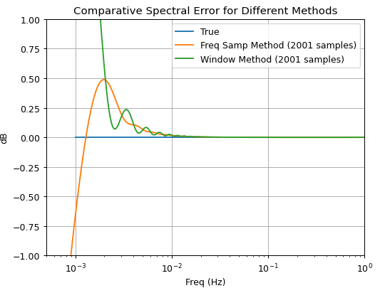
Comparative Spectral Error

The Python code used to create the filter coefficients using 'frequency sampling' is as follows:

import numpy as np
import scipy.signal as sig
import matplotlib.pyplot as plt
import scipy.fft as fft
fs = 2      
N = 1001        # number of discrete freqs (using odd number for symmetry)
a = 1.2566      # constant
b = 0.00078956  # constant

k = np.arange(1, (N-1)/2+1)  # frequency indices for pos frequencies
f = fs/N * k                 # frequencies at sampled locations

#The spectrum
G = np.zeros(N)
hw = int((N-1)/2)   # half-way 

# create positive frequencies
G[1:hw+1] = a / np.sqrt(b*f[:hw])
# create negative frequencies as symmetric spectrum
G[hw+1:] = G[1:hw+1][::-1]
# DC Bin
G[0]= G[1]

# Create time domain response using IDFT
win = sig.kaiser(len(G),12) 
coeff = fft.ifftshift(fft.ifft(G)) * win    

# Recreate spectrum (as DTFT) and plot
w, h = sig.freqz(coeff, worN=2**16)
plt.figure()
plt.semilogx(f, 20*np.log10(G), label="True")
plt.semilogx(fs/2 * w/np.pi, 20*np.log10(np.abs(h)), label="Freq Sampling") 

Closing Thoughts

This post has presented the corrected approach to the OP's approach of using the Frequency Sampling Method for determining the time response from a frequency response, and provided a comparison to the alternative Windowing Method (detailed nicely in MattL's answer).

I have also gained through working through the OP's question a deeper understanding of the Frequency Sampling Method, in that there are cases (this one!) where the method provides just as good of a result as the alternative Windowing Method without any downsides. In most use cases for Frequency Sampling that I was previously familiar with, notably whenever the target spectrum has an abrupt discontinuity, the frequency spectrum must be oversampled to significantly more samples in order to achieve the same performance as the Windowing Method. As MattL has pointed out to me in the past, this does NOT mean the resulting filter need be longer, since the derived time domain response from the Frequency Sampling Method can be truncated and windowed. I was hoping to demonstrate that point in this post but found out surprisingly the two approaches have the same performance in this case without the need for increasing the density of frequency samples. My suspicion is the smoothness of the OP's target spectrum given the $1/\sqrt{f}$ shape.

$\endgroup$
14
  • $\begingroup$ +1 This will probably work, provided we define some finite desired response at DC, because the original desired response goes to infinity as $\omega\to 0$. $\endgroup$
    – Matt L.
    Commented Jun 2, 2023 at 11:19
  • $\begingroup$ @MattL Good point, I set the DC bin to match the first bin. I didn't see a lot of sensitivity to variation so the actual value doesn't appear critical. With interest, I compared the results from this method to your method (see final plot). The Freq Sampling Method resulted in a lot less error than the Windowing Method you used which is not intuitive to me. I didn't even increase the freq grid further (2001 samples directly). Could there be an error in your impulse response or bin 0 value used? Or is my result what you would have expected? $\endgroup$ Commented Jun 4, 2023 at 5:22
  • $\begingroup$ (It occurs to me that this "better" result is due to the smoothness in the target frequency, so a unique case where Frequency Sampling is actually better without having to increase grid etc!) $\endgroup$ Commented Jun 4, 2023 at 11:04
  • 1
    $\begingroup$ As a conclusion I'd say that whenever an analytical solution is feasible and easy enough to compute, I'd go for that, plus windowing of course. Otherwise, frequency sampling (plus windowing) can be a good alternative, possibly with oversampling, depending on the desired function. $\endgroup$
    – Matt L.
    Commented Jun 5, 2023 at 10:17
  • 1
    $\begingroup$ @DanBoschen: Sure Kaiser is the more flexible window, so if I need that flexibility I'll definitely go for a Kaiser window. But in many of the practical cases I've come across, Hanning was good enough for me. $\endgroup$
    – Matt L.
    Commented Jun 6, 2023 at 9:44
6
$\begingroup$

As an alternative to the frequency sampling method discussed in Dan's answer, I will suggest another approach based on the analytical expression of the inverse discrete-time Fourier transform (IDTFT) of the desired frequency response. The resulting sequence can then be windowed and shifted such that the ideal response can be approximated by a linear-phase FIR filter. This is just the windowing method of filter design. Note that even though frequency sampling and windowing are usually not very popular for the design of frequency selective filters, they are very well suited for the approximation of smooth desired functions as the one given in the question.

In this answer it was mentioned that an analytical solution exists for the continuous Fourier transform, but that result cannot directly be used for a discrete-time implementation. Below I will derive the expression for the inverse discrete-time Fourier transform (IDTFT) of the desired response

$$G(\omega)=\frac{1}{\sqrt{|\omega|}}\tag{1}$$

Note that any desired scaling of $(1)$ can be directly applied to the IDTFT $g[n]$.

The IDTFT of $(1)$ is given by

$$g[n]=\frac{1}{2\pi}\int_{-\pi}^{\pi}\frac{e^{j\omega n}}{\sqrt{|\omega|}}d\omega=\frac{1}{\pi}\int_0^{\pi}\frac{\cos(\omega |n|)}{\sqrt{\omega}}d\omega$$

For $n\neq 0$ we obtain

$$\begin{align}g[n]&=\frac{1}{\pi \sqrt{|n|}}\int_0^{\pi |n|}\frac{\cos(x)}{\sqrt{x}}dx\\&=\frac{2}{\pi \sqrt{|n|}}\int_0^{\sqrt{\pi |n|}}\cos(x^2)dx\\&=\frac{2}{\sqrt{\pi}}\frac{C(\sqrt{\pi |n|})}{\sqrt{\pi |n|}},\qquad n\neq 0\tag{2}\end{align}$$

where $C(x)$ is the Fresnel integral $\int_0^x\cos(t^2)dt$.

For $n=0$ we obtain

$$g[0]=\frac{1}{\pi}\int_0^{\pi}\frac{d\omega}{\sqrt{\omega}}=\frac{2}{\sqrt{\pi}}\tag{3}$$

which also happens to be the limit of $(2)$ as $n\to 0$.

The IDTFT $g[n]$ is symmetrical and of infinite length. The corresponding filter is non-causal and unstable. In order to implement it approximately, we can apply a symmetrical window and then shift the response to the right such that the resulting filter is causal. Note that $g[n]$ decays only very slowly, so we have to use a rather long FIR filter to keep the approximation error small. However, if complexity and delay are of no concern, we can approximate the desired response as closely as we like.

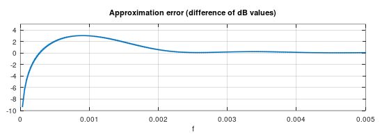
In the example below I designed an FIR filter with $2001$ taps according to above procedure using a Hanning window. The figure shows the approximation error defined as the difference of the designed FIR response (in dB) minus the ideal response (in dB). Note that only the frequency region very close to DC is shown, because the error is virtually zero for frequencies further away from DC.

enter image description here

Below is the Matlab/Octave code to compute the filter coefficients of the FIR filter:

M = 1000;
N = 2*M + 1;    % number of taps = 2001
n = (1:M)';
% express (cosine) Fresnel integral by error function
x = sqrt( pi * n );
E1 = erf( ( 1 + 1i ) / sqrt(2) * x );
E2 = erf( ( 1 - 1i ) / sqrt(2) * x );
C = real( .25 * sqrt( pi / 2 ) * ( 1 - 1i ) * ( E1 + 1i * E2 ) );
g = 2 / sqrt(pi) * C ./ x;
g = [ g(M:-1:1); 2/sqrt(pi); g ];
w = hanning( N );
gw = w .* g;
$\endgroup$
20
  • $\begingroup$ +1 Yes, mine may well work, but this is the better approach, similar to the reasons of my ingrained thinking to avoid "frequency sampling" for filter design when we can just work from samples of the impulse response directly (which by the way you helped me see cases where that can be useful to do and how to do that properly). However in that case it is further improved by windowing that impulse response in time. With the same logic, would windowing improve the result here further by reducing the edge effects? $\endgroup$ Commented Jun 3, 2023 at 1:38
  • $\begingroup$ @DanBoschen: This is just the windowing method for designing filters. I used a Hanning window (look at the code at the end of my answer). To me, the traditional windowing method and frequency sampling are very similar in the sense that in both cases you compute an inverse transform of the desired response. This inverse transform is then truncated (using a window) and made causal. If it's possible I compute the analytical solution, otherwise frequency sampling on a dense grid followed by windowing is also a good solution. $\endgroup$
    – Matt L.
    Commented Jun 3, 2023 at 8:57
  • $\begingroup$ Yes I see the windowing was used now, I had missed that. I may take back "this approach is better" now having compared the two (see bottom of my answer), where the Freq Sampling approach actually came up with a better spectral match given same number of samples used- which initially surprised me. Curious if it also makes sense to you? $\endgroup$ Commented Jun 4, 2023 at 11:06
  • 2
    $\begingroup$ Note that answers are not only for the OP but also for all future visitors. The answers here satisfy all levels of interest. You can just copy/paste the code, or you can learn how to derive the result, depending on your interest and level of understanding. $\endgroup$
    – Matt L.
    Commented Jun 11, 2023 at 10:14
  • 1
    $\begingroup$ @DanBoschen Apologies for delayed response. I appreciate the lively discussion on this question. In general I agree with that both answers were quite technical. But I also think they were helpful. I thought Dan's was the most helpful and used less jargon, so I've marked it as the "correct" answer. $\endgroup$
    – Darcy
    Commented Jun 14, 2023 at 20:13
3
$\begingroup$

If you want to get a real-valued $g(t)$, then its Fourier transform (FT) $G(ω)$ must be conjugate-symmetrical. So your expression of $G(ω)$ should be $G(ω)=\frac{a}{\sqrt{b|ω|}}$ after you set $\phi(ω)=0$. Otherwise, if $G(ω)=\frac{a}{\sqrt{bω}}$, it is impossible to get a real-valued $g(t)$ as its inverse fourier transform (IFT).

The IFT of $\frac{1}{\sqrt{|ω|}}$ has an analytic expression. That is,

$$IFT\{{\frac{1}{\sqrt{|ω|}}}\}=\frac{1}{\sqrt{|t|}}$$

You can use this result to directly get the expression of $g(t)$ in your case. Note that this is based on the definition of FT and IFT as

$$X(\omega)=\frac{1}{\sqrt{2\pi}}\int_{-\infty}^{\infty}x(t)e^{-j\omega t} \, \mathrm{d}t,$$

$$x(t)=\frac{1}{\sqrt{2\pi}}\int_{-\infty}^{\infty}X(\omega)e^{j\omega t} \, \mathrm{d}\omega.$$

If you are using a slightly different definition regarding the constants before the integral signs, there is a minor scaling adjustment.

Otherwise if you like, you may use ifft in MATLAB to obtain $g(t)$ numerically. You have to make sure to create a symmetric sequence of $G(\omega)$ before doing ifft in order to get correct result.

$\endgroup$
4
  • $\begingroup$ "you may use ifft" that's incorrect $\endgroup$ Commented Jun 2, 2023 at 19:51
  • 1
    $\begingroup$ @OverLordGoldDragon Would mind to tell me what is wrong ? Honestly, I already did it using ifft in MATLAB before I wrote the above answer. Of course, it is a numerical method to get a discrete sequence to represent the continuous function of $g(t)$. $\endgroup$
    – user295357
    Commented Jun 2, 2023 at 21:08
  • $\begingroup$ We can't just sample some $G(\omega)$ and iFFT to get $g(t)$. Aliasing, spacing, alignment. Yet, a $G(\omega)$ for which is is truer would probably be more helpful to OP. $\endgroup$ Commented Jun 11, 2023 at 11:47
  • 4
    $\begingroup$ @OverLordGoldDragon Thanks for your comment and reply. As I told you, I already did it in Matlab, and the plotted result is perfectly consistent with the analytical result. This is not to do IFFT on a measured or sampled data of $G(\omega)$, instead, this is to do IFFT of a clearly and analytically defined function of $G(\omega)$, so there is no such problems as aliasing, spacing and alignment Anyway, I respect your opinion. $\endgroup$
    – user295357
    Commented Jun 11, 2023 at 14:05

Your Answer

By clicking “Post Your Answer”, you agree to our terms of service and acknowledge you have read our privacy policy.

Not the answer you're looking for? Browse other questions tagged or ask your own question.