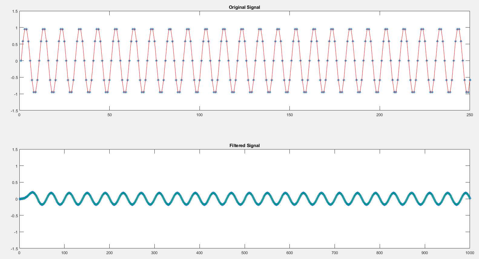
I first commented that a scaling by 4 is required but, as Marcus commented, we observe in the OP's code that such a scaling is already being done. I then replicated the OP's code as follows: (ordering the zero-insert operation properly in order to obtain any output)
fs = 1000;
t = 0:1/fs:0.5-1/fs;
sig1 = sin(2*pi*50*t);
x_up = zeros(1,sig_len*4);
x_up(1:4:len(sig1)*4)= 4*sig1(1:len(sig1));
fv = [8 12]/fs;

b = fir1(40,fv);

filt_sig = filter(b,1,x_up);
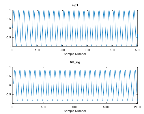
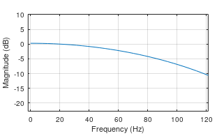
The level is slightly reduced, but nowhere near that in the OP's plot. Given the code as shown will not work, I suspect there are other differences between the code the OP posted and what was actually used (specifically I suspect the scaling by 4 was not actually done). The observed slightly reduced level is consistent with the suboptimal filtering used for interpolation, and consistent with the frequency response of the OP's interpolation filter:
freqz(b,1,512, 4000)
Zooming in on this passband response we observe the -1.4 dB attenuation at the 50 Hz signal:
An efficient interpolation filter can be designed using the least squares algorithm (firls in MATLAB, Octave and Python scipy.signal) that minimizes any loss or distortion in the passband and maximizes rejection only where it is needed- for example, if we assume a desired passband from DC to 50 Hz, then the only frequency bands where interpolation images will appear in the output signal after zero insert are from 975 to 1025 Hz and 1975 to 2000 Hz up to Nyquist (at the 4KHz output rate).
The following filter will provide nearly 100 dB rejection of the interpolation images and only requires 12 coefficients:
coeff = firls(12, [0 50 975 1025 1975 2000]/2000, [1 1 0 0 0 0]);
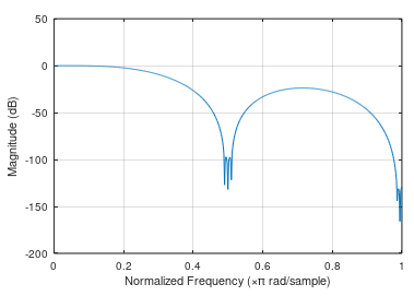
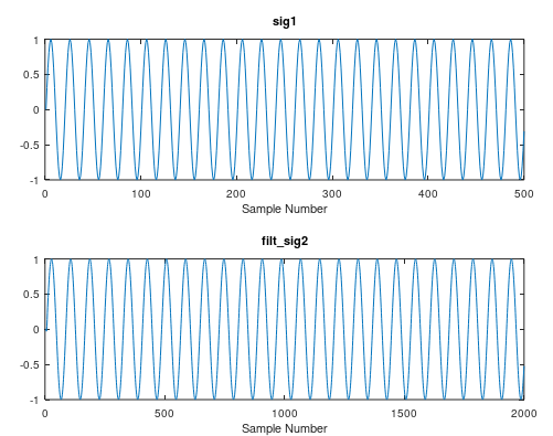
Filtering x_up with this new filter results in the updated plot below showing the original signal and the interpolated signal with minimum distortion. Further we would get such a clean result for any waveform in the DC to 50 Hz passband.
(See these other posts regarding polyphase implementations where this could be converted to 4 3-tap polyphase filters all running at the original 1 KHz rate!)
Prior response regarding amplitude scaling requirements with interpolation:
An amplitude change is expected with zero padding interpolation when passed through the same FIR filter for interpolation. An FIR filter is simply a weighted moving average, so we can intuitively see what happens if we consider a case of an FIR filter with unity gain coefficients and scale the output to normalize the gain of the filter. For a simple example consider a 4 tap FIR filter with unity gain coefficients:

The output is divided by 4 to be a true moving average, alternatively the coefficients could have been each scaled by 0.25. Either way we see in this case that the output signal will now match the scaling of the input signal when the signal is within the passband of the filter. In this case when we do the simplest case of a "DC" tone as a stream of ones the output will also converge to a stream of ones:
$$x[n] = [1, 1, 1, 1, 1, 1, \ldots]$$
We will get:
$$y[n] = [0.25, 0.5, 0.75, 1, 1, 1, 1, \ldots]$$
Now consider the same case with the input interpolated by 2 (for example), which is done by inserting s zero in between each input sample:
$$x_i[n] = [1, 0, 1, 0, 1, 0, \ldots]$$
We will get:
$$y_i[n] = [0.25, 0.25, 0.5, 0.5, 0.5, 0.5 \ldots]$$
The solution is to simply scale by $N$ where $N$ is the interpolation factor (with $N-1$ zeros inserted).



x_upas zeros, then overwrite every fourth elelemt withsig1. $\endgroup$