Biexponential (double exponential) convolution of a function

Question

Summary

I am trying to run a convolution on some data that was originally calculated from a deconvolution (so the reverse). However I'm not getting the expected graph.

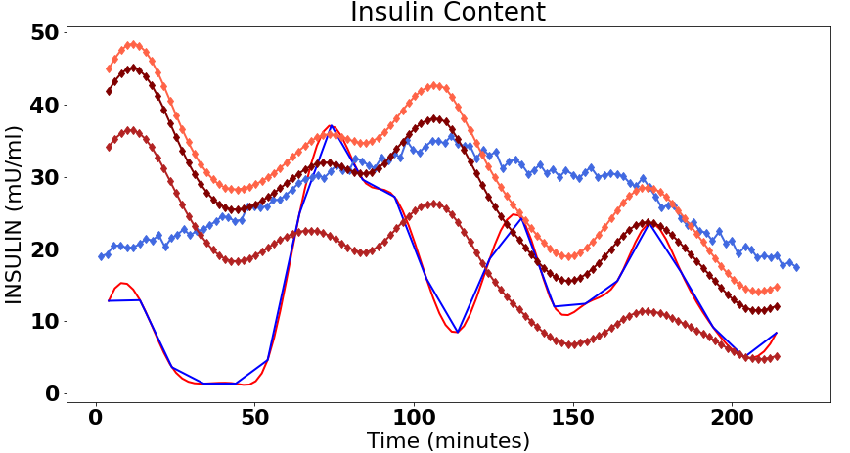
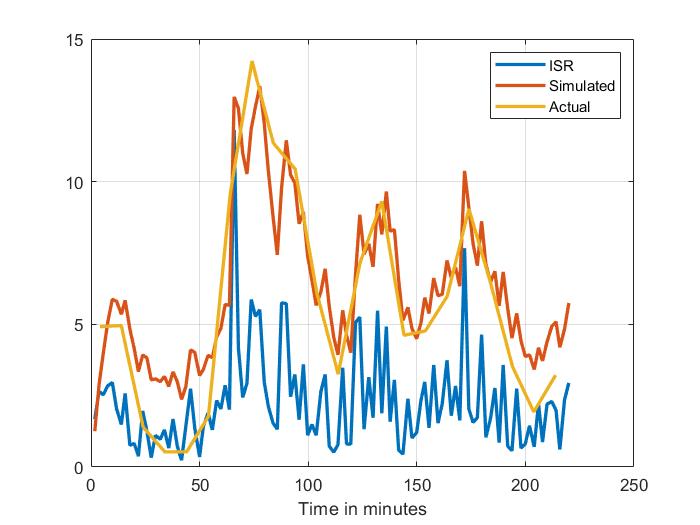
Blue is expected, red is a interpolated version of expected. Then the diamond lines are various convolutions with either or both of the two half lives active in the convolution.

Questions

1. Am I using the biexponential formula correctly? I think so because it matches the book for the two slopes being graphed.
2. The ISR was calculated from a deconvolution of the Insulin concentration then running a convolution on ISR should give the Insulin concentration, correct? I believe this is correct because "Computing the inverse of the convolution operation is known as deconvolution." from https://en.wikipedia.org/wiki/Convolution
3. Am I using the convolution function correctly? I assume not. Is this an issue of the 'window' of the function, trying to apply it over the full set of Y vs applying it to say 5 minutes of the ISR data at a time?

Data

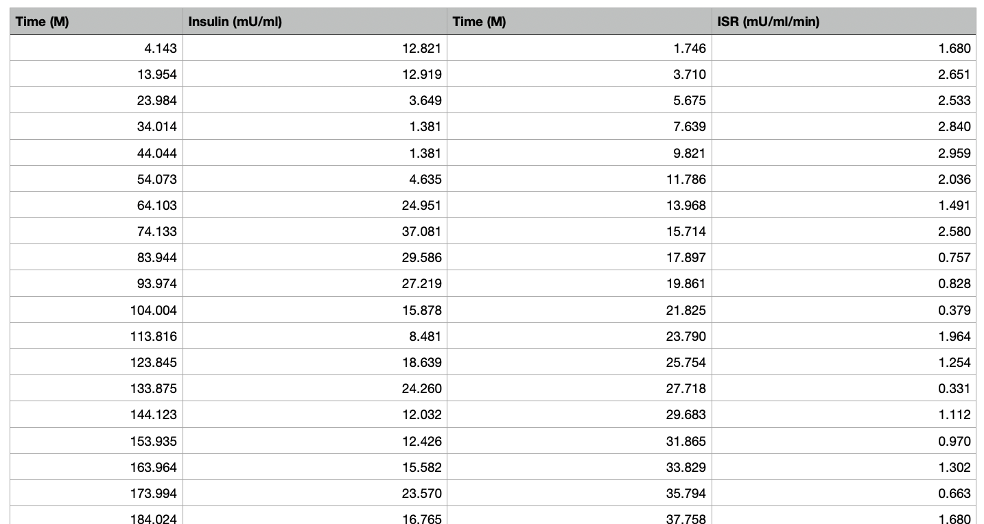
I have the following data that I extracted from a paper's (https://doi.org/10.2337/diabetes.51.2007.S258) graph (using https://apps.automeris.io/wpd/).

The data is:

1. Insulin concentration in mU/ml which was gathered experimentally.
2. Insulin secretion rate (ISR) in mU/ml/min which was calculated from the first data.

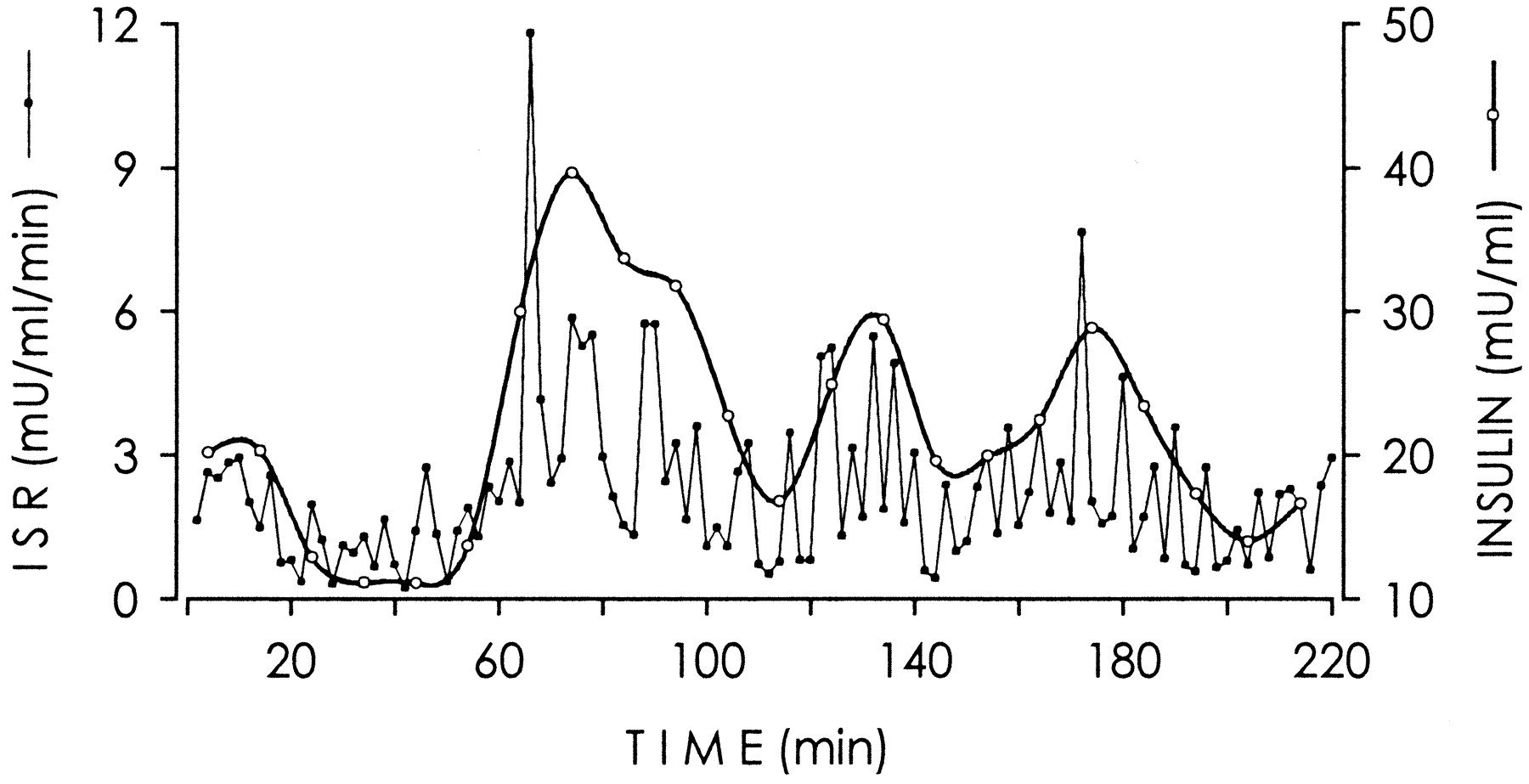Graph from https://diabetes.diabetesjournals.org/content/51/suppl_1/S258.figures-only

The ISR was calculated according to the paper,

A deconvolution method based on a biexponential disappearance rate of insulin, assuming half-lives for insulin of 2.8 and 5 min with a fractional slow component of 28% (19)

ref 19 is https://pubmed.ncbi.nlm.nih.gov/11134098/

and on the description of figure 2

ISR was estimated by deconvolution analysis from plasma insulin concentrations.

So because the ISR was calculated from a deconvolution then running a convolution on ISR should give the Insulin concentration, correct?

Formula

Using https://onlinelibrary.wiley.com/doi/pdf/10.1002/9780470126714.app4 it seems the formula is (other sources back this up 1, 2, 3, and page 40 formula 4 and 5)

$$ y=ae^{-bt} + ce^{-dt} $$

so I insert the specific values the paper mentions (I'm not 100% on what "fractional slow component" is see answer figured it out).

Note: First 0.28 is the fractional slow component and the second is 2.8 minutes.

$$ y=72\%e^{-log(2)t/5.0} + 28\%e^{-log(2)t/2.8} $$

so

$$ y=0.72e^{-log(2)t/5.0} + 0.28e^{-log(2)t/2.8} $$ Putting it together

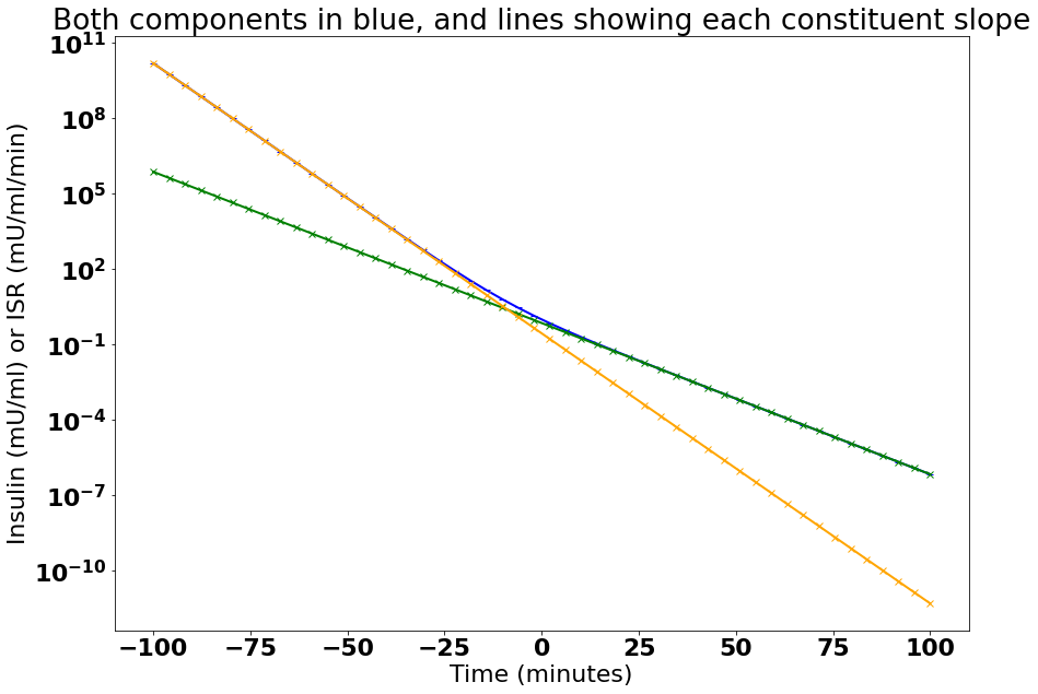
First I wanted to make sure I have the formula understood. So I graphed it on a semi-logy plot.

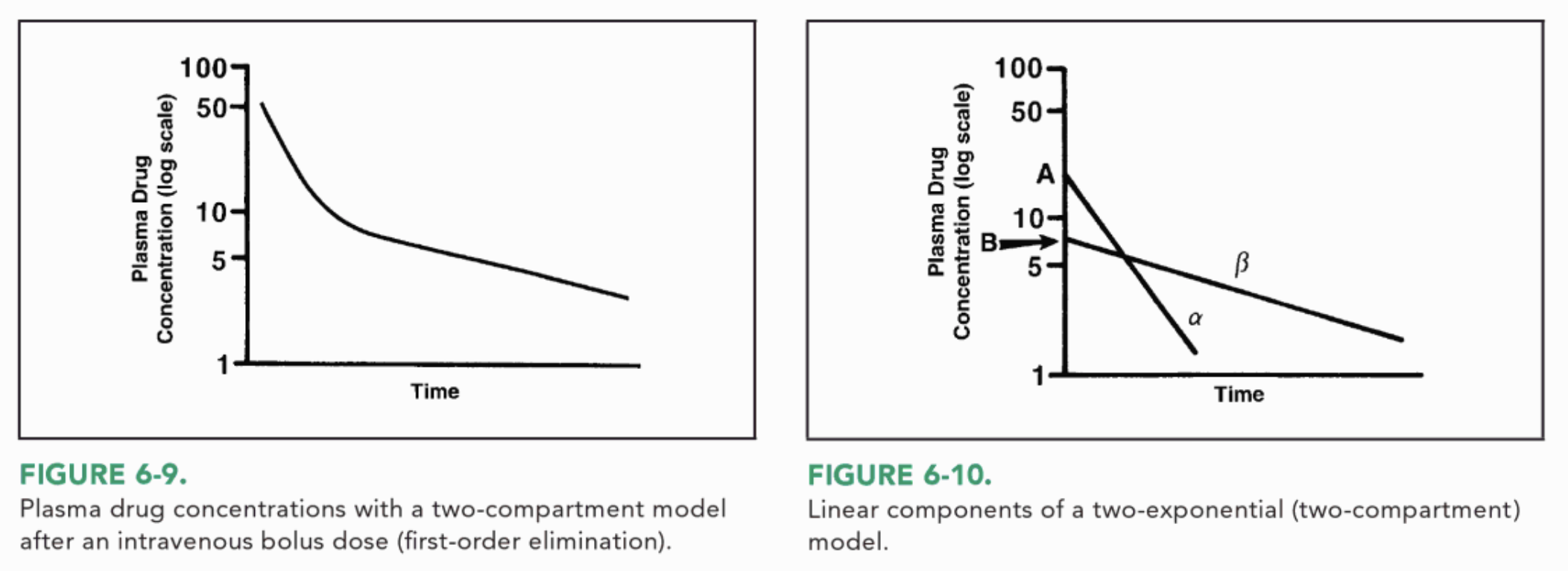
This is based off of Figure 6-9 on page 78 Concepts in Clinical Pharmacokinetics by By Joseph T. DiPiro

So it seems I have the correct formula I think

Running the convolution

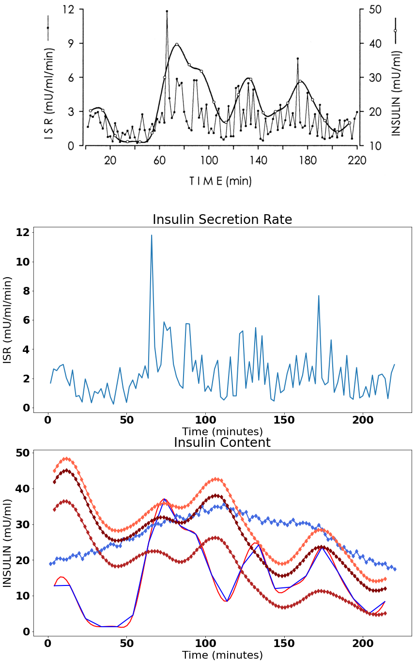
I get the following three graphs, first is a picture of the original. Second is the ISR data extracted from the graph, and the final graph has,

1. original insulin content in blue
2. interpolated version in red to 110 data points
3. three convolutions with either both biexponential slopes or just one of them in red
4. and a convolution of the original data in royal blue.

Full Code

import numpy as np
import pandas
import matplotlib.pyplot as plt
import scipy
from scipy.interpolate import splrep, splev
from scipy.optimize import curve_fit
import urllib.request
import scipy as sp

# set matplotlib display properties
import matplotlib as mpl
mpl.rcParams['lines.linewidth'] = 2
font = {'family' : 'normal',
        'weight' : 'bold',
        'size'   : 22}

mpl.rc('font', **font)


# data from figure 2
# https://diabetes.diabetesjournals.org/content/51/suppl_1/S258.figures-only

#data_ins = pandas.read_csv("Insulin.dat", header = None, delimiter = '\t')

#data_isr = pandas.read_csv("ISR.dat", header = None, delimiter = '\t')

insulin_json = '{"0":{"0":4.143,"1":13.954,"2":23.984,"3":34.014,"4":44.044,"5":54.073,"6":64.103,"7":74.133,"8":83.944,"9":93.974,"10":104.004,"11":113.816,"12":123.845,"13":133.875,"14":144.123,"15":153.935,"16":163.964,"17":173.994,"18":184.024,"19":194.054,"20":203.865,"21":213.895},"1":{"0":12.821,"1":12.919,"2":3.649,"3":1.381,"4":1.381,"5":4.635,"6":24.951,"7":37.081,"8":29.586,"9":27.219,"10":15.878,"11":8.481,"12":18.639,"13":24.26,"14":12.032,"15":12.426,"16":15.582,"17":23.57,"18":16.765,"19":9.172,"20":5.03,"21":8.383}}'
isr_json = '{"0":{"0":1.746,"1":3.71,"2":5.675,"3":7.639,"4":9.821,"5":11.786,"6":13.968,"7":15.714,"8":17.897,"9":19.861,"10":21.825,"11":23.79,"12":25.754,"13":27.718,"14":29.683,"15":31.865,"16":33.829,"17":35.794,"18":37.758,"19":39.722,"20":41.687,"21":43.651,"22":45.833,"23":47.798,"24":49.98,"25":51.726,"26":53.909,"27":55.873,"28":57.837,"29":59.802,"30":61.766,"31":63.73,"32":65.913,"33":67.877,"34":69.841,"35":71.806,"36":73.77,"37":75.734,"38":77.698,"39":79.772,"40":81.627,"41":83.81,"42":85.774,"43":87.738,"44":89.921,"45":91.885,"46":93.849,"47":95.813,"48":97.778,"49":99.742,"50":101.706,"51":103.671,"52":105.853,"53":107.817,"54":109.673,"55":111.746,"56":113.71,"57":115.893,"58":117.639,"59":119.603,"60":121.786,"61":123.75,"62":125.714,"63":127.897,"64":129.861,"65":131.935,"66":133.899,"67":135.972,"68":137.718,"69":139.683,"70":141.647,"71":143.611,"72":145.903,"73":147.758,"74":149.94,"75":151.905,"76":153.651,"77":155.615,"78":157.798,"79":159.762,"80":161.726,"81":163.909,"82":165.873,"83":167.837,"84":169.802,"85":171.984,"86":173.948,"87":175.913,"88":177.877,"89":179.841,"90":181.806,"91":183.988,"92":185.952,"93":187.917,"94":189.772,"95":191.845,"96":193.81,"97":195.992,"98":197.956,"99":199.921,"100":201.885,"101":204.067,"102":206.032,"103":207.887,"104":209.96,"105":212.143,"106":214.107,"107":215.853,"108":218.036,"109":220.0},"1":{"0":1.68,"1":2.651,"2":2.533,"3":2.84,"4":2.959,"5":2.036,"6":1.491,"7":2.58,"8":0.757,"9":0.828,"10":0.379,"11":1.964,"12":1.254,"13":0.331,"14":1.112,"15":0.97,"16":1.302,"17":0.663,"18":1.68,"19":0.734,"20":0.237,"21":1.42,"22":2.746,"23":1.349,"24":0.355,"25":1.42,"26":1.893,"27":1.302,"28":2.331,"29":2.036,"30":2.864,"31":2.012,"32":11.811,"33":4.166,"34":2.438,"35":2.935,"36":5.87,"37":5.278,"38":5.515,"39":2.97,"40":2.13,"41":1.538,"42":1.325,"43":5.751,"44":5.728,"45":2.462,"46":3.243,"47":1.657,"48":3.598,"49":1.112,"50":1.491,"51":1.112,"52":2.651,"53":3.243,"54":0.734,"55":0.521,"56":0.781,"57":3.479,"58":0.805,"59":0.805,"60":5.065,"61":5.254,"62":1.325,"63":3.148,"64":1.728,"65":5.479,"66":1.882,"67":4.923,"68":1.586,"69":3.053,"70":0.592,"71":0.45,"72":2.391,"73":1.018,"74":1.207,"75":2.331,"76":2.982,"77":1.373,"78":3.574,"79":1.538,"80":2.225,"81":3.74,"82":1.799,"83":2.84,"84":1.633,"85":7.669,"86":2.036,"87":1.562,"88":1.728,"89":4.639,"90":1.041,"91":1.716,"92":2.769,"93":0.852,"94":3.574,"95":0.734,"96":0.568,"97":2.746,"98":0.663,"99":0.805,"100":1.444,"101":0.71,"102":2.225,"103":0.876,"104":2.201,"105":2.296,"106":1.988,"107":0.615,"108":2.367,"109":2.947}}'
data_ins = pandas.read_json(insulin_json)
data_isr = pandas.read_json(isr_json)


def main():

    new_length = 110
    new_x = np.linspace(data_ins.iloc[:,0].min(), data_ins.iloc[:,0].max(), new_length)
    new_y = sp.interpolate.interp1d(data_ins.iloc[:,0], data_ins.iloc[:,1], kind='cubic')(new_x)

    # function of a biexponential decay
    # https://swharden.com/blog/2020-09-24-python-exponential-fit/
    # https://www.graphpad.com/guides/prism/latest/curve-fitting/reg_exponential_decay_2phase.htm
    # https://pharmacy.ufl.edu/files/2013/01/two-compartment-model.pdf
    # http://websites.umich.edu/~elements/07chap/html/07prof5.htm
    #
    # "This type of behavior is observed, for example, in the radioactive decay 
    # of a mixture of two nuclides with different half-lives, one short 
    # lived and the other relatively longer-lived."
    # y=ae^(-bt) +ce^(-dt)
    # https://onlinelibrary.wiley.com/doi/pdf/10.1002/9780470126714.app4
    #
    # A short introduction to pharmacokinetics
    # R. URSO, P. BLARDI, G. GIORGI
    # https://www.europeanreview.org/wp/wp-content/uploads/6.pdf
    # https://www.certara.com/knowledge-base/simplifying-deconvolution/
    def biExp(x, a, b, c, d):
        return (a * np.exp(x*b)) + (c * np.exp(x*d))



    ################################################################
    # 2.8 and 5.0 minutes and 0.28 percent from                    #
    # Ultradian Oscillations of Insulin Secretion in Humans        #
    # -------------------------------------------------------------#
    # "A deconvolution method based on a biexponential             #
    # disappearance rate of insulin, assuming half-lives           #
    # for insulin of 2.8 and 5 min with a                          #
    # fractional slow component of 28% (19)"                       #
    # ref 19 is https://pubmed.ncbi.nlm.nih.gov/11134098/          #
    # https://doi.org/10.2337/diabetes.51.2007.S258                #
    # -------------------------------------------------------------#
    # Direct measurement of pulsatile insulin secretion from       #
    # the portal vein in human subjects                            #
    # -------------------------------------------------------------#
    # "a biexponential insulin disappearance model in the          #
    # systemic circulation, consisting of earlier directly         #
    # estimated half-lives of 2.8 and 5.0 min and a                #
    # fractional slow component of 0.28 in healthy fasting humans" #
    # https://pubmed.ncbi.nlm.nih.gov/11134098/ (ref 19 above)     #
    # -------------------------------------------------------------#
    # In humans at least 75% of insulin secretion arises from      #
    # punctuated insulin secretory bursts                          #
    # -------------------------------------------------------------#
    # "insulin kinetics of 2.8 min (first half-life),              #
    # 5.0 min (second half-life), and                              #
    # a fractional slow component of 0.28"                         #
    # https://pubmed.ncbi.nlm.nih.gov/9374676/                     #
    # -------------------------------------------------------------#

    a = 1 - 0.28 # I assume from graphpad link that speaks of percent
    b = -np.log(2)/5.0 # 1/minutes
    c = 0.28 # fractional slow component of 0.28?
    d = -np.log(2)/2.8 # 1/minutes

    # See if the exponential function looks correct compared to 
    # Concepts in Clinical Pharmacokinetics
    # By Joseph T. DiPiro
    # Page 78 Figure 6-9
    fig, ax = plt.subplots(1, figsize=(14,10))
    ax.semilogy()
    ax.title.set_text("Both components in blue, and lines showing each constituent slope")
    ax.yaxis.set_label_text("Insulin (mU/ml) or ISR (mU/ml/min)")
    ax.xaxis.set_label_text("Time (minutes)")

    x_window = 100
    x_values = np.linspace(-x_window, x_window)
    # graph both
    ax.plot(x_values, biExp(x_values, a,b,c,d), 
        marker = '_', color = 'blue')

    # only graph the fast part (first)
    ax.plot(x_values, biExp(x_values, a,b,0,d), 
        marker = 'x', color = 'green')

    # only graph the slow part (second)
    ax.plot(x_values, biExp(x_values, 0,b,c,d), 
        marker = 'x', color = 'orange')



    # now calculate the actual convolution
    fig, ax = plt.subplots(3, figsize=(14,24))

    # create a file-like object from the url
    f = urllib.request.urlopen("https://diabetes.diabetesjournals.org/content/diabetes/51/suppl_1/S258/F2.large.jpg?width=800&height=600&carousel=1")

    # turn off axis since they really don't add much
    ax[0].set_axis_off()
    # read the image file in a numpy array
    img = plt.imread(f, format='jpg')
    ax[0].imshow(img, cmap='gray')


    # display ISR which was calculated orginally from the deconvolution
    # of measured Insulin Concentration
    ax[1].title.set_text("Insulin Secretion Rate")
    ax[1].yaxis.set_label_text("ISR (mU/ml/min)")
    ax[1].xaxis.set_label_text("Time (minutes)")
    ax[1].plot(data_isr.iloc[:,0], data_isr.iloc[:,1])


    # display non convolution version
    # (needs some smoothing)
    ax[2].title.set_text("Insulin Content")
    ax[2].yaxis.set_label_text("INSULIN (mU/ml)")
    ax[2].xaxis.set_label_text("Time (minutes)")
    ax[2].plot(new_x, new_y, color = "red")
    ax[2].plot(data_ins.iloc[:,0], data_ins.iloc[:,1], color = "blue")

    # convolution of ISR
    ax[2].plot(data_isr.iloc[:,0], np.convolve(data_isr.iloc[:,1],
        biExp(data_isr.iloc[:,1], a,b,c,d), mode = "same")/5, # bi exponential function
    color = "royalblue", marker = "d")

    ax[2].plot(new_x, np.convolve(new_y,
        biExp(new_y, a,b,c,d), mode = "same") / 10, # bi exponential function
    color = "maroon", marker = "d")

    # break them down to components
    ax[2].plot(new_x, np.convolve(new_y,
        biExp(new_y, 0,b,1,d), mode = "same") / 10, # bi exponential function
    color = "firebrick", marker = "d")


    ax[2].plot(new_x, np.convolve(new_y,
        biExp(new_y, 1,b,0,d), mode = "same") / 10, # bi exponential function
    color = "tomato",  marker = "d")


if __name__ == "__main__":
    main()

CSV Export of the data

Time (M),Insulin (mU/ml),Time (M),ISR (mU/ml/min)
4.143,12.821,1.746,1.680
13.954,12.919,3.710,2.651
23.984,3.649,5.675,2.533
34.014,1.381,7.639,2.840
44.044,1.381,9.821,2.959
54.073,4.635,11.786,2.036
64.103,24.951,13.968,1.491
74.133,37.081,15.714,2.580
83.944,29.586,17.897,0.757
93.974,27.219,19.861,0.828
104.004,15.878,21.825,0.379
113.816,8.481,23.790,1.964
123.845,18.639,25.754,1.254
133.875,24.260,27.718,0.331
144.123,12.032,29.683,1.112
153.935,12.426,31.865,0.970
163.964,15.582,33.829,1.302
173.994,23.570,35.794,0.663
184.024,16.765,37.758,1.680
194.054,9.172,39.722,0.734
203.865,5.030,41.687,0.237
213.895,8.383,43.651,1.420
,,45.833,2.746
,,47.798,1.349
,,49.980,0.355
,,51.726,1.420
,,53.909,1.893
,,55.873,1.302
,,57.837,2.331
,,59.802,2.036
,,61.766,2.864
,,63.730,2.012
,,65.913,11.811
,,67.877,4.166
,,69.841,2.438
,,71.806,2.935
,,73.770,5.870
,,75.734,5.278
,,77.698,5.515
,,79.772,2.970
,,81.627,2.130
,,83.810,1.538
,,85.774,1.325
,,87.738,5.751
,,89.921,5.728
,,91.885,2.462
,,93.849,3.243
,,95.813,1.657
,,97.778,3.598
,,99.742,1.112
,,101.706,1.491
,,103.671,1.112
,,105.853,2.651
,,107.817,3.243
,,109.673,0.734
,,111.746,0.521
,,113.710,0.781
,,115.893,3.479
,,117.639,0.805
,,119.603,0.805
,,121.786,5.065
,,123.750,5.254
,,125.714,1.325
,,127.897,3.148
,,129.861,1.728
,,131.935,5.479
,,133.899,1.882
,,135.972,4.923
,,137.718,1.586
,,139.683,3.053
,,141.647,0.592
,,143.611,0.450
,,145.903,2.391
,,147.758,1.018
,,149.940,1.207
,,151.905,2.331
,,153.651,2.982
,,155.615,1.373
,,157.798,3.574
,,159.762,1.538
,,161.726,2.225
,,163.909,3.740
,,165.873,1.799
,,167.837,2.840
,,169.802,1.633
,,171.984,7.669
,,173.948,2.036
,,175.913,1.562
,,177.877,1.728
,,179.841,4.639
,,181.806,1.041
,,183.988,1.716
,,185.952,2.769
,,187.917,0.852
,,189.772,3.574
,,191.845,0.734
,,193.810,0.568
,,195.992,2.746
,,197.956,0.663
,,199.921,0.805
,,201.885,1.444
,,204.067,0.710
,,206.032,2.225
,,207.887,0.876
,,209.960,2.201
,,212.143,2.296
,,214.107,1.988
,,215.853,0.615
,,218.036,2.367
,,220.000,2.947

Answer 1

All right, there are few issues to tackle here.

The ISR was calculated from a deconvolution of the Insulin concentration then running a convolution on ISR should give the Insulin concentration, correct?

Maybe. Deconvolution is an ill defined problem. Typically it only works if both system and the data are reasonably well behaved and even then there is typically significant loss of information and data.

Am I using the biexponential formula correctly? I think so because it matches the book for the two slopes being graphed.

I don't believe you do. An exponential decay can be written as $$h(t) = e^{-at}$$ Note that the constant has units of "one over time" or frequency. If you have half life of 5 minutes, the corresponding decay curve would be $$h_5(t) = e^{-\log(2)\frac{t}{5min}}$$ The half life time is in the denominator and you need a factor of $\log (2)$ to get it actual to "half" instead of $e^{-1}$

You also have an obvious scaling issue. The IRS peaks at 10-ish whereas the Insulin goes up to 40. The bi-exponential model alone can't account for that gain difference.

Once you fix the time constants and the scaling, things look a little better

The simulated Insulin is still a way more wiggly, but that's also a consequence of the actual Insulin being down sampled by a factor of 5. In general, the sample rates feel very low for that type of data and there is likely significant aliasing in there as well.

Here is the Matlab code. I imported the data by copying pasting the text file into a spreadsheet and saving it as an .CSV file

%% script
[a,b,c] = xlsread('foo.csv');  % read CSV file
%% eliminate the empty cells
t1 = a(:,1); % time
t1(isnan(t1)) = [];
x1 = a(:,2); % insulin
x1(isnan(x1)) = [];
t2 = a(:,3);  % time
x2 = a(:,4);  % IRS

%% buid the impules response and filter the data
h = .72*exp(-log(2)/5.*t2)+.28*exp(-log(2)/2.8.*t2);
% filter with the first 40 taps, that seems plenty
y = filter(h(1:40),1,x2);


%% plot it
clf;
plot(t2,[x2 y]);
hold on
% scale factor: match the RMS
x1s = x1./rms(x1)*rms(y);
plot(t1,x1s);
grid on
xlabel('Time in minutes');
legend('ISR','Simulated','Actual');
h = get(gca,'Children'); set(h,'Linewidth',2);

Answer 2

I did want to note that I figured out what fractional slow component was. Following the references

Ultradian Oscillations of Insulin Secretion in Humans
Chantal Simon and Gabrielle Brandenberger
Ref 19
-----------------------
Direct measurement of pulsatile insulin secretion from the portal vein in human subjects
S H Song  1 , S S McIntyre, H Shah, J D Veldhuis, P C Hayes, P C Butler
Ref 19
https://watermark.silverchair.com/jcem4491.pdf
Ref 6
-----------------------
1995: Pulsatile insulin secretion accounts for 70% of total insulin secretion during fasting
 NIELS PORKSEN, STEPHEN MUNN, JEFFERY STEERS, STEPHEN VORE, JOIIANNES VELDHUIS, AND PETER BUTLER
Ref 30
https://pubmed.ncbi.nlm.nih.gov/7573425/
-----------------------
1987: The pituitary gland secretes in bursts: Appraising the nature of glandularsecretoryimpulsesbysimultaneousmultiple-parameter deconvolution of plasma hormone concentrations
JOHANNES D. VELDHUIS*t, MARK L. CARLSONt, AND MICHAEL L. JOHNSON
https://www.pnas.org/content/84/21/7686
https://www.pnas.org/content/pnas/84/21/7686.full.pdf

In the last paper from 1987 it has "TheE(t- z)term can be described reasonably by either a one- or two-component model with two half-lives, HL1 and HL2, and a fraction, f, which describes their relative contributions:"

$$ E(t-z) = fe^{-(0.693(t-z)/HL1])} + (1-f)e^{-0.693(t-z)/HL2} $$

This cites ref 3 which is Lakowicz,J.R.(1983)Principles of Fluorescence Spectroscopy (Plenum, New York), pp. 65-87.