Wouldn't this be equivalent to discarding all those frequencies in the input layer?
No, it won't for 2 facts:
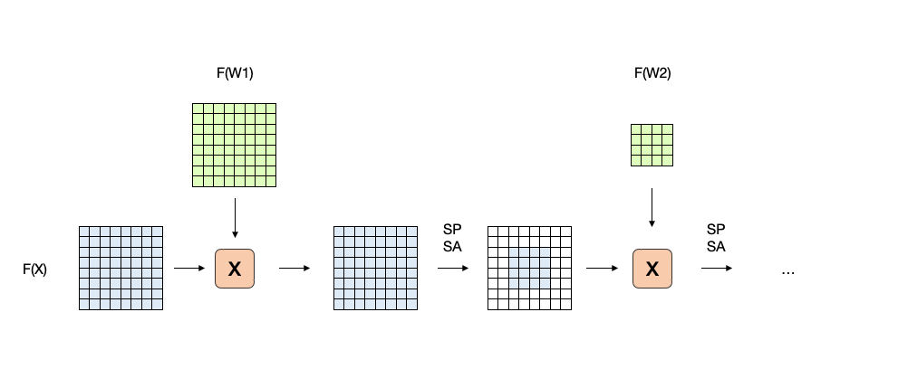
Just like a CNN isn't a linear regression due to having non linear function in between. So the Activation Layers on the frequency domain mean things are not propagated linearly in the forward pass.
The filters are adaptive (Learned). Namely each layer will have a different response on the middle (Low Frequencies).
Basically what we see is cascaded low pass filters with non linear activation in between.
The way I see it, the major advantage doing it so:
- There is a better understanding what we should pull and what not. Low frequency details are explicitly preserved.
- Computations are done with multiplications vs. convolutions. So for some dimensions combination it might be faster.
Example
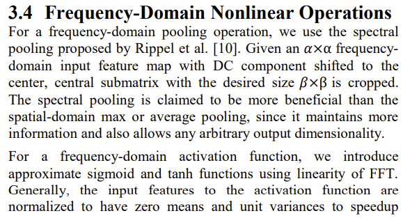
In order to show, let's just apply a toy example using the building blocks of Design of an Energy Efficient Accelerator for Training of Convolutional Neural Networks Using Frequency Domain Computation.
Specifically how they describe the Spectra Pooling and Spectral Activation (See Section 3.4):
The code I created (1D Toy Example):
%<! Question 76875

clear();
close('all');

% Choosing Odd length for simplicity.
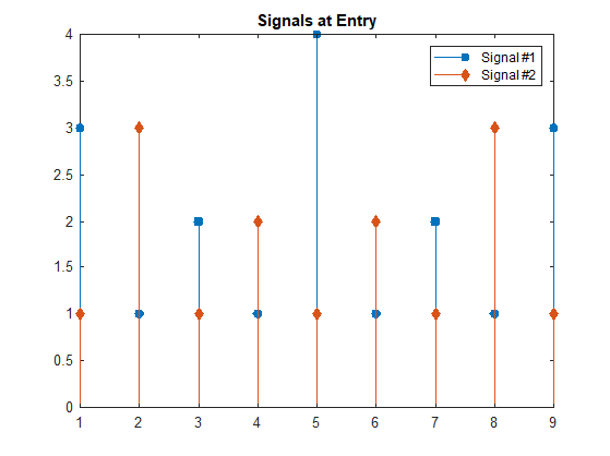
vS1 = [3; 1; 2; 1; 4; 1; 2; 1; 3];
vS2 = [1; 3; 1; 2; 1; 2; 1; 3; 1];

vF1 = [0; 0.25; 0.5; 0.75; 1; 0.75; 0.5; 0.25; 0];
vF2 = [1; 0.75; 0.5; 0.25; 0; 0.25; 0.5; 0.75; 1];


figure();
hStemObj = stem([vS1, vS2], 'filled');
set(hStemObj(2), 'marker', 'd');
title({['Signals at Entry']});
legend({['Signal #1'], ['Signal #2']});

figure();
hStemObj = stem([vF1, vF2], 'filled');
set(hStemObj(2), 'marker', 'd');
title({['Filters']});
legend({['Filter at Stage #1'], ['Filter at Stage #2']});

vS1F1 = vS1 .* vF1;
vS1F1 = SpectralActivation(vS1F1, 1); %<! Apply activation (Sigmoid)
vS1F1 = SpectralPooling(vS1F1, 3); %<! Remove 1 from each side

vS2F1 = vS2 .* vF1;
vS2F1 = SpectralActivation(vS2F1, 1); %<! Apply activation (Sigmoid)
vS2F1 = SpectralPooling(vS2F1, 3); %<! Remove 1 from each side

figure();
hStemObj = stem([vS1F1, vS2F1], 'filled');
set(hStemObj(2), 'marker', 'd');
title({['Signals After First Filter + Spectral Activation + Spectral Pooling']});
legend({['Signal #1'], ['Signal #2']});

vS1F2 = vS1F1 .* vF2;
vS1F2 = SpectralActivation(vS1F2, 1); %<! Apply activation (Sigmoid)
vS1F2 = SpectralPooling(vS1F2, 2); %<! Remove 1 from each side

vS2F2 = vS2F1 .* vF1;
vS2F2 = SpectralActivation(vS2F2, 1); %<! Apply activation (Sigmoid)
vS2F2 = SpectralPooling(vS2F2, 2); %<! Remove 1 from each side

figure();
hStemObj = stem([vS1F2, vS2F2], 'filled');
set(hStemObj(2), 'marker', 'd');
title({['Signals After Second Filter + Spectral Activation + Spectral Pooling']});
legend({['Signal #1'], ['Signal #2']});


figure();
hStemObj = stem([vS1F2 ./ vS1, vS2F2 ./ vS2], 'filled');
set(hStemObj(2), 'marker', 'd');
title({['Equivalent Filter (Output ./ Input)']});
legend({['Signal #1'], ['Signal #2']});


function [ vO ] = SpectralPooling( vI, kernelRadius )

    numSamples  = size(vI, 1);
    centerIdx   = ceil(numSamples / 2); %<! Assuming Odd

    vIdx = (centerIdx - kernelRadius):(centerIdx + kernelRadius);

    vO = zeros(numSamples, 1);
    vO(vIdx) = vI(vIdx);

end

function [ vO ] = SpectralActivation( vI, sigSlope )

    % Normalization: Non Linear Operation
    vO = (vI - mean(vI)) / std(vI);
    % In paper approximated by a linear function
    vO = 1 ./ (1 + exp(-sigSlope * vO));

end
So we have 2 input signals (Imagine this is their spectrum):
I chose 2 filters:
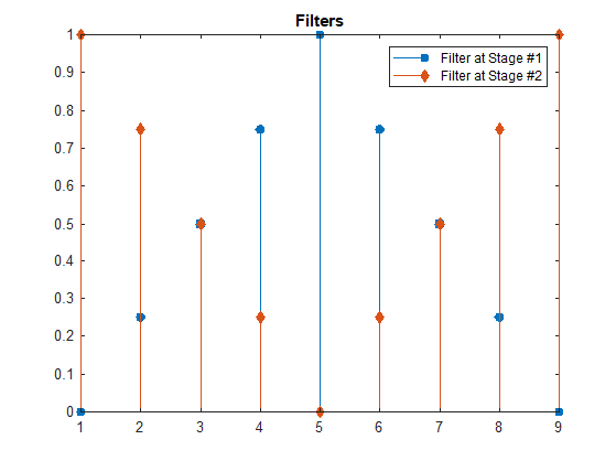
In practice the filters are learned. Hence they don't have any special meaning.
Now, let's see the result of the 2 signals when they go through Filter 1 (Since we're in frequency domain the filter is element wise multiplication) + Spectral Activation (Normalization + Sigmoid) + Spectral Pooling:
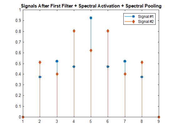
We can see that indeed only the center part of the signal is kept. Yet the values of each are not proportional. We'll have a deeper look after the next stage - Filter 2 + Spectral Activation (Normalization + Sigmoid) + Spectral Pooling:
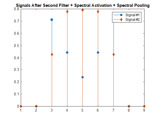
Now, we can see even more narrower yet we can see each signal was filtered completely different. This is due to the non linear steps.
Let's do one more thing. If this could be replaced just by an LPF (With finite support, so it would do some "Pooling") then the ratio of the output to input of both signals would be the same (This what would have happened in an LTI system). Let's examine this ratio:
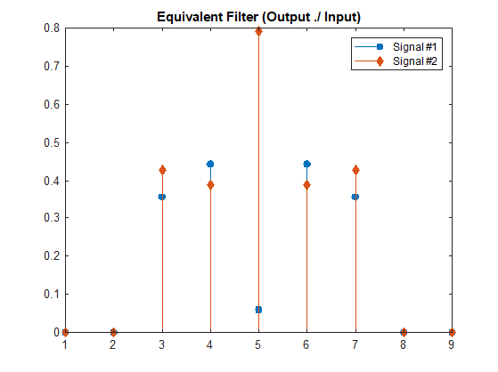
We can see that each signal was processed completely differently.
So, indeed as written to begin with, though the system discard high frequencies, it alters the remaining frequencies in a non linear manner. Hence it can not be replaced by a multiplication by a rectangular in the frequency domain.
Update
At Frequency Pooling: Shift Equivalent and Anti Aliasing Downsampling they are trying to build operators which downsample with keeping the shift invariant property in tact.

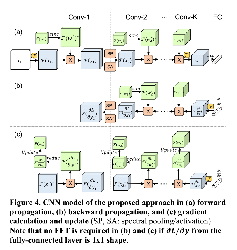
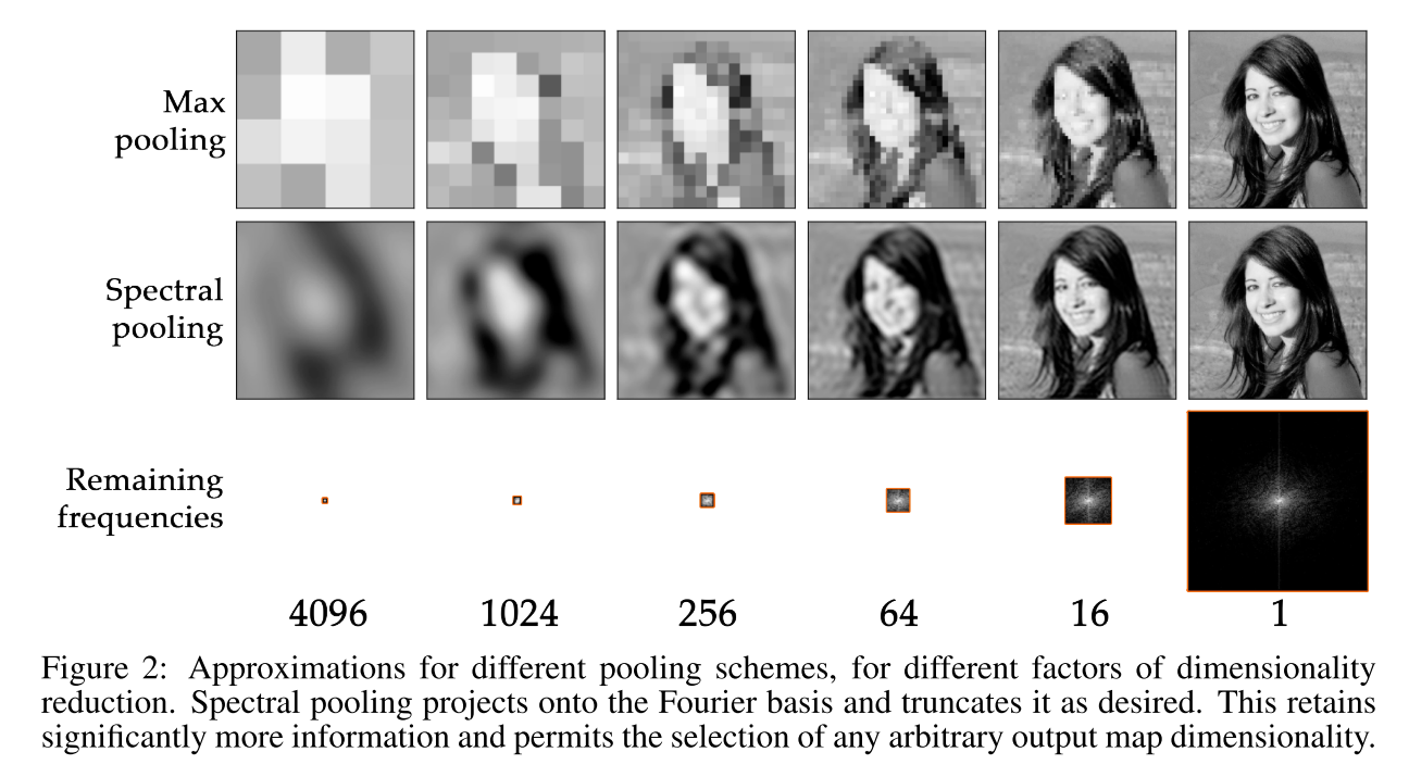


Design of an energy efficient accelerator for training of convolutional neural networks using frequency Domain Computation, the author mention that if the output is size $1 \times 1$, in which theiFFToutput would be the same as its input. The issue is, given the spectral pooling applied in such way, the output would seem to rely only on the DC of the input. $\endgroup$