I am trying to plot windows of acquired data from an LSL-compatible system. For the example below, let's consider 1-second window of a 64 channel EEG system. In practice, I use shorter 0.2-window, but the problematic behavior is present also with 1-second window.
The acquired data is a numpy array of shape (samples, channels), thus in this example, with a 512 Hz sampling frequency: (512, 64).
Before plotting the data, it has to be preprocessed with a bandpass filter. Let's consider a [1, 40] Hz bandpass filter:
from scipy.signal import butter

lowcut = 1
highcut = 40
fs = 512

low = lowcut / (0.5 * fs)
high = highcut / (0.5 * fs)
sos = butter(4, [low, high], btype='band', output='sos', fs=fs)
As each window will be plot on the same expanding graph, the initial and final conditions of each window are required. Thus, the zi parameter is passed to scipy.signal.sosfilt() to retrieve the zf final conditions. The system is initialized with a resting state initial condition.
zi = np.zeros((sos.shape[0], 2, n)) # n = 64 - number of channels
To filter the data, I then apply:
data_filtered, zf = sosfilt(sos, data, 0, zi)
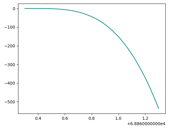
I don't see what I am doing wrong, and yet the output is diverging. By the way, I tried order 2, 4 and 6; and it does change the output but still diverge.
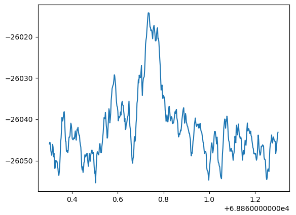
Inputted window of 1 channel:
Output window of the same channel:
After some research, I believe I should not specify the fs parameter to scipy.signal.butter() when passing the cutting frequencies as normalized from 0 to 1, where 1 is the Nyquist frequency. Nevertheless, the output is different but still diverging.
sos = butter(2, [1, 40], btype='band', output='sos', analog=False, fs=fs)


