Flipping of x axis values when the Fourier Transform is compared to the FFT

Question

EDITED 3-Jun-20

I have a lorentzian lineshape $$ f(z) = \frac{1+iz}{R(1+z^2)} \qquad (1)$$ where $$ z=\frac{-2\pi(f - F0)}{R} \qquad (2)$$ and $ R $ is the decay rate, $ f $ is the frequency, $ F0 $ is the peak frequency.

The time domain function should be $$ \exp(2\pi iF0t)\exp(-Rt)/Fs \qquad (3)$$ Where $ Fs $ is the sampling frequency (and is used as a scaling factor).

This FT pair has been obtained from the response here with a few simplifications, and i'm fairly certain its correct as i've gone through and derived it, and checked it against other derivations of the Lorentzian FT.

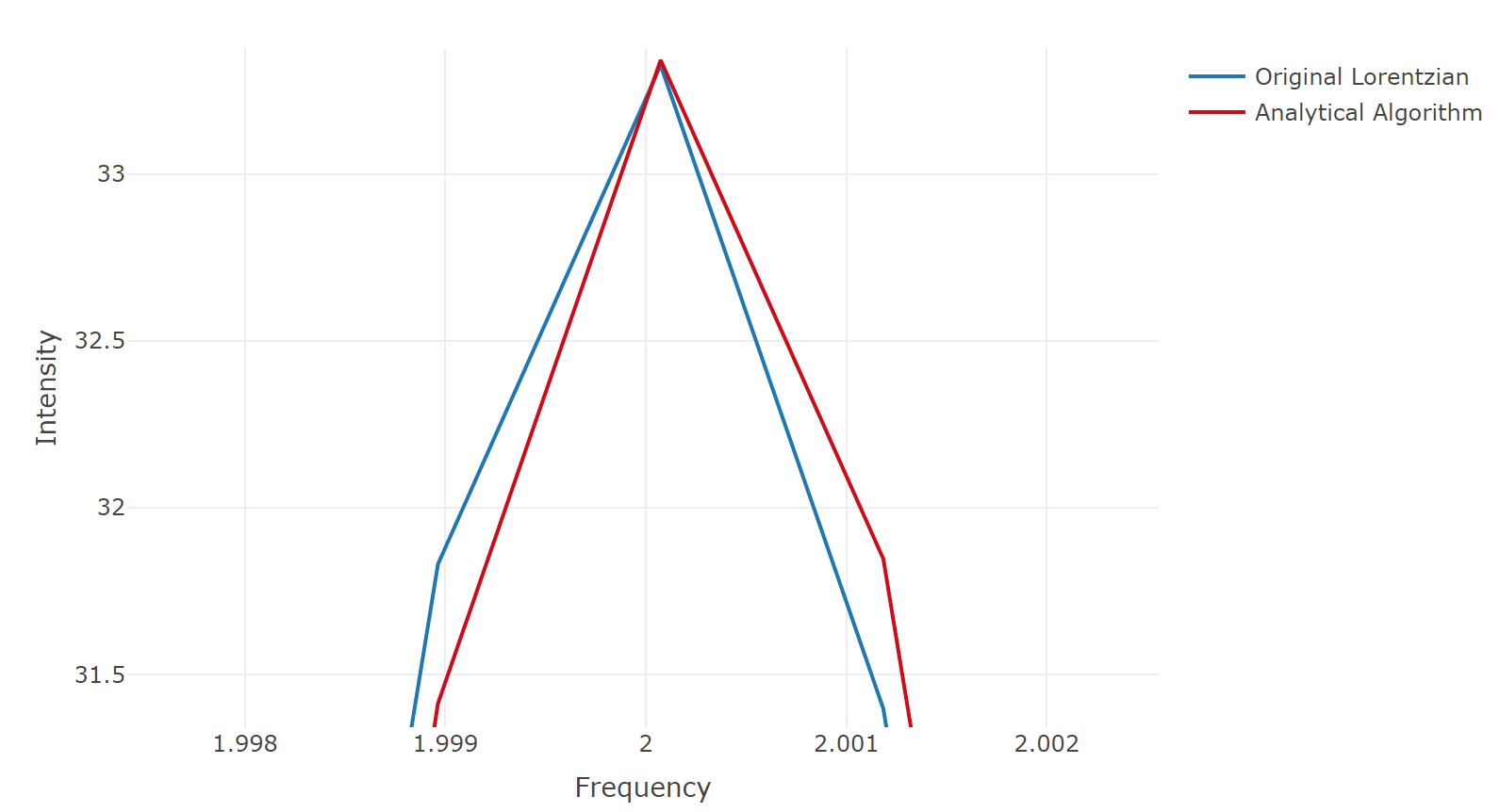
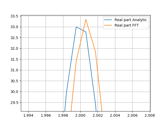
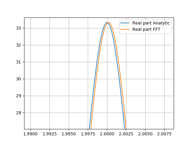
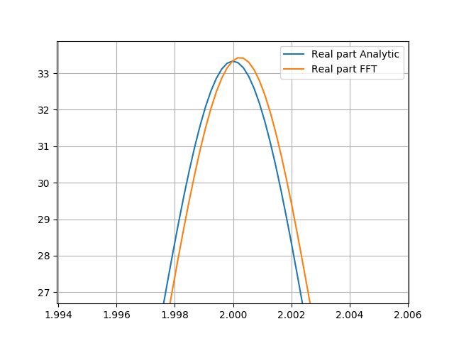
I am comparing the analytical Fourier Transform with the Fast Fourier Transform. I want to be able to obtain the original Lorentzian lineshape (equation 1) when i take the FFT of equation 3. I understand that there are differences between the two, and that there will be errors (truncation and/or aliasing), however when i compare them, the analytical FT result appears to be mirrored. This is easy to see when the peak tips are compared. I can write an algorithm to flip the x axis values and shift the peak back to where it should be, however i'm wondering why this flip happens. What is the theoretical basis? Is there a way to solve this without reversing and shifting each x axis value?

Please find the script showing the mirroring below.

library(SynchWave)
library(RcppFaddeeva)
library(plotly)

# 1) Lineshape parameters
Fs <- 30            # sampling frequency Hz
F0 <-  2            # resonance frequency
f_length <- 27000   # number of samples
A <- 1              # Peak intensity (Amplitude)
R <- 0.03           # Decay rate

# 2) Frequency data ---------------------------------------------
# Creating the frequency axis
f <- seq(0, Fs, length.out = f_length)

# The lorentz frequency lineshape
z <- -2*pi*(f - F0) / R
LL <- complex(r = 1, i = z)/(1+z^2)/R

# 3) Creating Time function ------------------------------------------
# Time axis
t <- seq(0, f_length/Fs, length.out = f_length)

# Ideal lorentz time lineshape
ft <- A*exp(complex(i = 2*pi*F0*t))*exp(-R*t)/Fs

#-------------------------------------------------------------
# 4) Checking for accuracy
x <- list(
  # X axis title
  title = "Frequency",
  titlefont = "f"
)
y <- list(
  # Y axis title
  title = "Intensity",
  titlefont = "f"
)

p <- plot_ly(x = f, y = Re(LL), mode = "lines", type = "scatter", name = "Original Lorentzian") %>%
     add_trace(x = f, y = Re(fft(ft)), mode = "lines", name = "Analytical Algorithm", line = list(color = 'rgb(205, 12, 24)')) %>%
     layout(xaxis = x, yaxis = y)
show(p)

and the script with the rudimentary flipping

library(SynchWave)
library(RcppFaddeeva)
library(plotly)

# 1) Lineshape parameters
Fs <- 30            # sampling frequency Hz
F0 <-  2            # resonance frequency
f_length <- 27000   # number of samples
A <- 1              # Peak intensity (Amplitude)
R <- 0.03           # Decay rate

# 2) Frequency data ---------------------------------------------
# Creating the frequency axis
f <- seq(0, Fs, length.out = f_length)

# The lorentz frequency lineshape
z <- -2*pi*(f - F0) / R
LL <- complex(r = 1, i = z)/(1+z^2)/R

# 3) Creating Time function ------------------------------------------
# Time axis
t <- seq(0, f_length/Fs, length.out = f_length)

# Ideal lorentz time lineshape
ftna <- A*exp(complex(i = 2*pi*(Fs-F0)*t))*exp(-R*t)/Fs
ftnew <- fft(ftna)
bot <- (Fs-F0)/Fs*f_length - F0/Fs*f_length
bot <- round(bot) + 2
ft <- ftnew[bot:(f_length-1)]
ft <- append(ft, ftnew[1:bot] , f_length)- min(Re(ftnew[1:bot]))

#-------------------------------------------------------------
# 4) Checking for accuracy
x <- list(
  # X axis title
  title = "Frequency",
  titlefont = "f"
)
y <- list(
  # Y axis title
  title = "Intensity",
  titlefont = "f"
)

p <- plot_ly(x = f, y = Re(LL), mode = "lines", type = "scatter", name = "Original Lorentzian") %>%
  add_trace(x = f, y = Re((ft)), mode = "lines", name = "Analytical Algorithm", line = list(color = 'rgb(205, 12, 24)')) %>%
  layout(xaxis = x, yaxis = y)
show(p)

Answer 1

This just seems like an error due to the finite number of samples you have.

You would get better results if you just increased the number of samples (make f_length <- 100000 for example).

Increasing the number of samples will improve your resolution in the frequency domain. Implicitly, you are also observing your signal for a longer time.

You will have to decide the tradeoff between these two.

---

I ran a Python script to display the same.

f_length is 27000.

f_length is 100000.

---

You could also reduce your sampling frequency and keep the number of samples the same. Since most of the signal energy is present around $f_o=2$, you could make $f_s=5$. Keep in mind, even here you are implicity observing the continuous-time signal for longer but at a lower sampling rate.

f_length is 27000, Fs is 5.

---

Hope this helped.