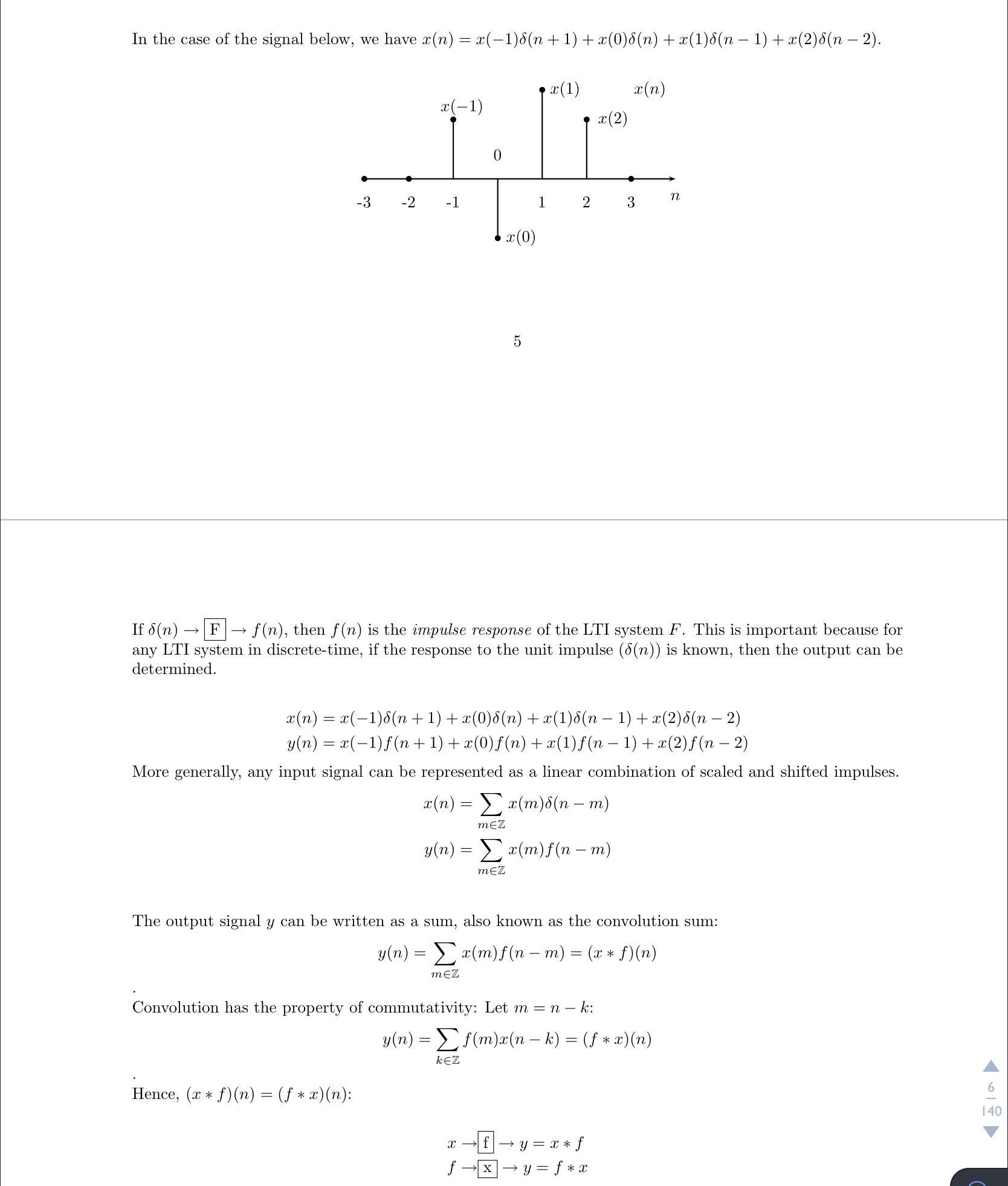
Going over some notes on LTI systems and I’m quite confused about how knowing the impulse response of a system allows us to recover the systems’ response to any signal. In the textbook screenshot below, it looks like they just replaced the Dirac deltas with $f$ when defining $y(n)$.
2 Answers
(Adapted from this answer on dsp.SE)
The reason that the impulse response (also called the unit pulse response for discrete-time systems) determines the output for arbitrary input $x$ to an LTI system is that
The output of a linear time-invariant system in response to input $x$ is the sum of scaled and time-delayed versions of the impulse response.
This is because of the linear property of the system: if the response to input signal $x_i$ is $y_i$, then the response to input $x_1+x_2+ x_3 + \cdots$ is $y_1+y_2 + y_3 + \cdots$. So, let's decompose the input signal $x$ into a sum of scaled unit pulse signals. The system response to the unit pulse signal $\cdots, ~0, ~0, ~1, ~0, ~0, \cdots$ is the impulse response or pulse response $$h[0], ~h[1], \cdots, ~h[n], \cdots$$ and so by the scaling property the single input value $x[0]$, or, if you prefer $$x[0](\cdots, ~0, ~0, ~1, ~0,~ 0, \cdots) = \cdots ~0, ~0, ~x[0], ~0, ~0, \cdots$$ creates a response $$x[0]h[0], ~~x[0]h[1], \cdots, ~~x[0]h[n], \cdots$$
Similarly, the single input value $x[1]$ or creates $$x[1](\cdots, ~0, ~0, ~0, ~1,~ 0, \cdots) = \cdots ~0, ~0, ~0, ~x[1], ~0, \cdots$$ creates a response $$0, x[1]h[0], ~~x[1]h[1], \cdots, ~~x[1]h[n-1], x[1]h[n] \cdots$$ Notice the delay in the response to $x[1]$. We can continue further in this vein, but it is best to switch to a more tabular form and show the various outputs aligned properly in time. We have $$\begin{array}{l|l|l|l|l|l|l|l} \text{time} \to & 0 &1 &2 & \cdots & n & n+1 & \cdots \\ \hline x[0] & x[0]h[0] &x[0]h[1] &x[0]h[2] & \cdots &x[0]h[n] & x[0]h[n+1] & \cdots\\ \hline x[1] & 0 & x[1]h[0] &x[1]h[1] & \cdots &x[1]h[n-1] & x[1]h[n] & \cdots\\ \hline x[2] & 0 & 0 &x[2]h[0] & \cdots &x[2]h[n-2] & x[2]h[n-1] & \cdots\\ \hline \vdots & \vdots & \vdots & \vdots & \ddots & \\ \hline x[m] & 0 &0 & 0 & \cdots & x[m]h[n-m] & x[m]h[n-m+1] & \cdots \\ \hline \vdots & \vdots & \vdots & \vdots & \ddots \end{array}$$ The rows in the above array are precisely the scaled and delayed versions of the impulse response that add up to the response $y$ to input signal $x$.
So, we see that if we know the impulse response of an LTI system, we can figure out the response of the LTI system to any arbitrary signal $x$. We don't need any additional information about the LTI system beyond the impulse response.
I think about this in terms of an impulse containing content at all frequencies, so if you know how the system responds to an impulse, you have a complete description of its response.
If you're comfortable with Laplace transforms, we can also say that the transfer function for a system can be computed by taking the Laplace transform of the impulse response - just jumping from the time domain to the z-domain.
More generally, you can also say that every input can be expressed as a sum of impulses. As a result, knowing how the system responds to an impulse allows you to establish how it responds to any arbitrary input. To do this in the time domain, you can convolve the input signal with the system's impulse response.

