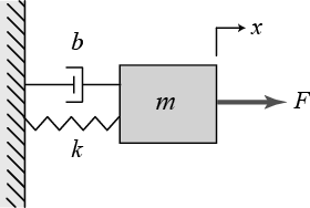
The mass-spring-damper combination is an LTI system described by the following continuous-time linear differential equation
$$ \ddot{x} = - \frac{k}{m} x - \frac{b}{m} \dot{x} + \frac{1}{m} u $$
where $u$ is the deterministic input force (N), $k$ is the spring constant (N/m) and $b$ is the damping coefficient (N.s/m).
Assuming two states as the position $x(t)$ and the velocity $\dot{x}(t)$; $X = [x , \dot{x}]^T$, and assuming a single measurement as the position $x(t)$ and assuming no process noise, and scalar deterministic input $u$ only added to the process equation, then the continuous-time linear dynamic system process and measurement equations for the Kalman filter can be written as
$$ \dot{X} = F X + G u $$
$$ y = H X + v $$
where
$$
F = \begin{bmatrix}
0 & 1 \\
-\frac{k}{m} & -\frac{b}{m}
\end{bmatrix}
$$
is the system dynamics matrix,
$$
G = \begin{bmatrix}
0 \\
1/m
\end{bmatrix}
$$
is the deterministic input matrix,
$$
H = \begin{bmatrix}
1 & 0
\end{bmatrix}
$$
is the measurement matrix, $v(t)$ is the measurement noise.
The first step in the derivation of the discrete Kalman filter is the discretization of the associated matrices by first finding the fundamental matrix $\Phi(t)$ which is given by :
$$ \Phi(t) = \mathcal{L}^{-1} \{ (s I - F)^{-1} \} $$
where $s$ is the complex variable of the Laplace transform.
For the given $F$, the fundamental matrix is found to be:
$$
\Phi(t) = e^{\frac{-b}{2m}t}
\begin{bmatrix}
\cos(\omega t) + \frac{b}{2m\omega } \sin(\omega t) & \sin(\omega t) / \omega \\
-\frac{k}{m\omega } \sin(\omega t) & \cos(\omega t) - \frac{b}{2m\omega } \sin(\omega t)
\end{bmatrix}\\
$$
where $\omega = \frac{\sqrt{4mk-b^2}}{2m}$.
Then the discrete fundamental matrix of the Kalman filter is found from $\Phi_k = \Phi(T)$ where $T$ is the sampling period.
$$
\Phi_k = e^{\frac{-b}{2m}T}
\begin{bmatrix}
\cos(\omega T) + \frac{b}{2m\omega } \sin(\omega T) & \sin(\omega T) / \omega \\
-\frac{k}{m\omega } \sin(\omega T) & \cos(\omega T) - \frac{b}{2m\omega } \sin(\omega T)
\end{bmatrix}\\
$$
We should also find the discrete versions of $H$ and $G$ which are found as $H_k = H = [1 , 0]$ and
$$G_k = \int_0^T \Phi(t) G dt .$$
By the help of a symbolic integration package (such as provided by MATLAB) one can compute the discrete deterministic input matrix $G_k$ as
$$
G_k = \frac{e^{aT}}{m (a^2+w^2)}
\begin{bmatrix}
\frac{a}{\omega} \sin(\omega T)-\cos(\omega T) + e^{-aT} \\
a (1-\omega) (\cos(\omega T)-1) + (a^2+ \omega) \sin(\omega T)
\end{bmatrix}\\
$$
where $ a = -b/2m $ and $\omega = \sqrt{4km-b^2}/2m$ as before.
After having found all the necessary discrete matrices $\Phi_k$, $G_k$, $H_k$ we can setup the discrete Kalman process and measurement equations through which the recursive solution can be applied.
$$X[n] = \Phi_k X[n-1] + G_k u[n]$$
$$ y[n] = H_k X[n] + v[n]$$
where $u[n]$,$v[n]$ and $y[n]$ are sampled versions of deterministic input, measurement noise and measurement respectively, and $X[n]$ is the sampled version of the state vector.
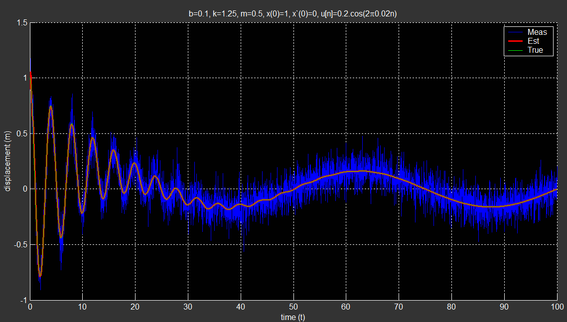
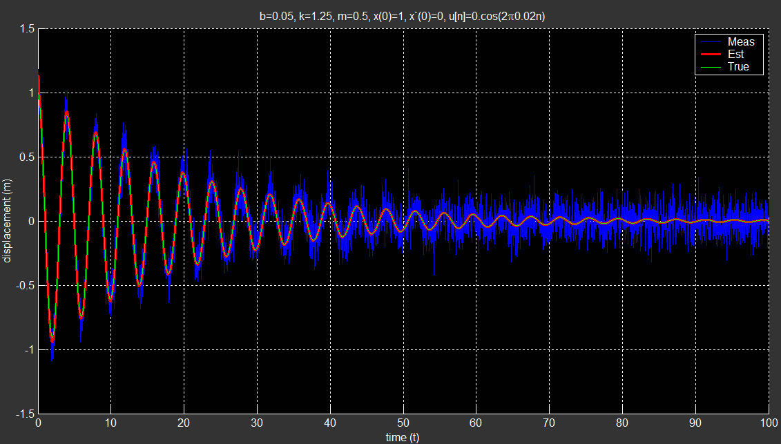
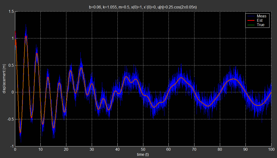
Then you will apply the Kalman recursion to estimate the states. Below are some simulation results from a MATLAB implementation of the associated Kalman filter. In the simulation, the true signal is generated by solving the associated ODE with a simple Runge-Kutta numerical method. Eventhough it's not required for this LTI system whose analytical solution is already available, it'll be helpful to use a numerical method later if more complicated (nonlinear) differential equations are encountered.


In this simulation, the model was exact. And therefore it's a little trivial. For more realistic applications, one should either replace the linear differential equation with more realistic nonlinear ones hence change the model and/or apply process noise to compansate for the lack of exact process model information.

