Why do additional harmonics arise after the filter bank?

Question

I'm trying to implement direct implementation of MDCT filter bank. So, some additional artefacts have appeared after all of the routines.

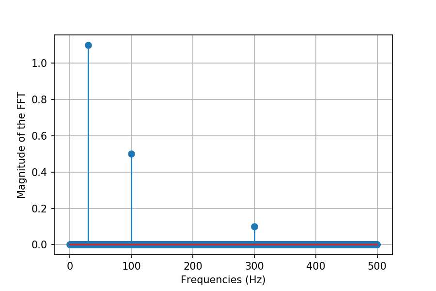
The spectrum of the initial signal looks like:

import numpy as np
import matplotlib.pyplot as plt

N = 8 #subbands
L = 2*N

h = np.zeros((L,1)) #skeleton for window function
for n in range(2*N-1):
    h[n] = np.sin((np.pi / (2 * N)) * (n + 0.5)) #window function

w = [30, 100, 300]
a = [1.1, .5, .1]
x = 0

t = np.array([i for i in range(1,3001)])/1000
for idx in range(len(w)):
    x = x + a[idx]*np.sin(2*np.pi*w[idx]*t)

FFT = np.fft.fft(x)
amps = np.abs(FFT) / (len(FFT) / 2)
fs = 1 / (t[1]-t[0])
f = fs*np.array([i for i in range(int(len(x)))]) / len(x)

plt.subplots(1, 1, figsize=(6, 4), dpi=150)
plt.stem(f[:int(len(f)/2)], amps[:int(len(f)/2)])
plt.ylabel('Magnitude of the FFT')
plt.xlabel('Frequencies (Hz)')
plt.grid(True)
plt.show()

# Analysis
H = np.zeros((N,L)) #skeleton for analisis H matrix
pr = (L+len(x)-1) #lengh (number of coloumn) of signal after convolution
Analysis_Mat = np.zeros((N,pr)) #skeleton for matrix after convolution
for k in range(N): #rows
    for n in range(L): #coloumns
        H[k,n] = h[n]*np.cos((np.pi/N)*(k+0.5)*(n+0.5-(N/2))) #analysis H matrix
    Analysis_Mat[k,:] = np.convolve(x,H[k,:]) #convolution

# Downsampling
M = int(Analysis_Mat.shape[1] / N) #number of samles that sould be stay after downsampling
cutmat = int(np.floor(M)*N) #number of rows that sould follow to downsampln block (cut rows that are not fold to N)

Analysis_Mat_DS = np.zeros((N, M))
Analysis_Mat = Analysis_Mat[:, :cutmat]

for k in range(N):
    Analysis_Mat_DS[k, :] = Analysis_Mat[k,::N]

# Upsampling


Analysis_Mat_US = np.zeros((N, Analysis_Mat_DS.shape[1]*N)) #skeleton for signal that should be after upsampling
for n in range(Analysis_Mat_DS.shape[1]):
    Analysis_Mat_US[:,0+N*n] = Analysis_Mat_DS[:, n]

# Synthesis

R = L + Analysis_Mat_US.shape[1] - 1 #legth of signal (number o rows) that should be after convolution 
Syntesis_Mat = np.zeros((N,R)) #skeleton for signal that should be after convolution 
G = (np.fliplr(H))/(N/2) #Synthesis matrix
for k in range(N):
    Syntesis_Mat[k,:] = np.convolve(Analysis_Mat_US[k,:], G[k,:]) #convolution
y = np.sum(Syntesis_Mat, axis=0)

FFT = np.fft.fft(y)
amps = np.abs(FFT) / (len(FFT) / 2)
fs = 1 / (t[1]-t[0])
f = fs*np.array([i for i in range(int(len(x)))]) / len(x)

plt.subplots(1, 1, figsize=(6, 4), dpi=150)
plt.stem(f[:int(len(f)/2)], amps[:int(len(f)/2)])
plt.ylabel('Magnitude of the FFT')
plt.xlabel('Frequencies (Hz)')
plt.grid(True)
plt.show()

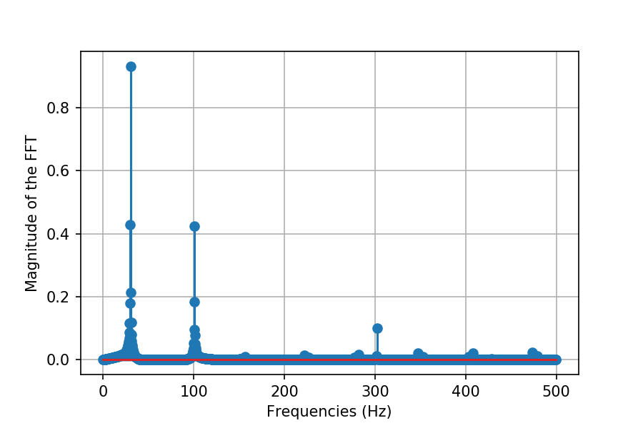
However, the reconstructed spectrum looks like:

Is it OK? Is there a mistake in my script or I don't understand the theory (or both)?

Can anybody help me with this issue?