4
$\begingroup$

I want to run a numerical simulation of a system (eg first order low pass filter) that is stimulated with a photocurrent-like signal. My preferred language is Python.

I'm failing to understand how to generate a proper time series for the photocurrent with a consistent noise power, especially when the photocurrent becomes very small.

Let's assume:

  • simulation interval time is dT
  • the mean photocurrent is I
  • q is the elementary charge
  • T is the time series length

In my understanding there are two main ways to model the photocurrent time series.

A) I calculate the average number of electrons and use this number to generate a poisson time series that I convert back into current

N = I * dT / q # mean number of electrons in interval dT
N_ts = np.random.poisson(N,int(T/dT)) # electrons time series
I_ts = N_ts * q / dT # resulting photocurrent time series

The problem I have with this is that if I becomes small enough then average number of electrons per dT is very low and when I draw samples from the distribution it behaves like a quantum current (some samples will have 0,1,2,3,.. electrons). Is this quantization a corrected model or is it a limitation of it? What is the meaning of dT in this case? Is it some sort of averaging? Should the dT be increased to avoid the quantization? If I increase dT, how much should it be increased? Does a change in dT change the noise power of a Poisson time series? How is dT related to the noise bandwidth of the signal? How can I rescale the noise after a dT change to maintain the same input noise power?

B) A second approach could be to avoid the photon counting and directly model a photocurrent time series drawing samples from a normal distribution with $\mu_I = I$ and $ \sigma_I = \sqrt{2qIB} $ However, what is the correct bandwidth to use in this case? Is it 1/(2*dT) because I'm assuming the sampling frequency is two times the noise bandwidth? A problem with modeling using a normal distribution is that if dT=1E-6 and I<1.602E-13 then $\sigma_I=\mu_I$, which means that if I draw samples from such distribution I might end up drawing negative currents. The normal distribution is not a good approximation of a Poissonian distribution for small currents. Should I use a lognormal distribution instead?

Are these approaches fundamentally correct? How do they differ from each other? Is there an equivalence between the two? Does Physics come actually into play with quantization when considering very small currents or is it an artifact of the modeling?

$\endgroup$
5
  • $\begingroup$ there's is quite a lot of signal simulation questions in there that make a lot of sense in the context of this site, but I think the central questions you're asking are all physical. That would be relatively off-topic here, so instead of an answer, let me just give a comment: Yes, light has this wave-particle dualism. In the intensity distribution ("statistics for arbitrarily long observations") it behaves like a wave – exposing properties like diffraction, refraction, interference. When it comes to energy delivery, it acts like particles – like quantums of energy being delivered. $\endgroup$ Commented Apr 27, 2019 at 7:09
  • $\begingroup$ so, that's the physical basis which I'd assume was the whole point of your simulation to show – if this is news to you, get a book about modern physics! $\endgroup$ Commented Apr 27, 2019 at 7:10
  • 2
    $\begingroup$ I'm aware of the wave-particle representation for photons and I understand that the background of this question is physics related. But this doesn't make all the underlying signal-related question less worth of an answer. I could still break the question down into valid signal processing questions like "What is the bandwidth of a sampled shot noise in the calculation of its noise power" or "how does the noise power of a sampled Poisson process changes with sampling time". They would just lack the bigger picture, which I think helps framing the problem. $\endgroup$
    – Knyq
    Commented Apr 29, 2019 at 16:11
  • $\begingroup$ I would welcome references if there is any that treat the problem in question with clear answers. $\endgroup$
    – Knyq
    Commented Apr 29, 2019 at 16:15
  • $\begingroup$ I definitely like the approach of painting the bigger picture! As said in my commentsw, there's a lot of good signal processing questions in there, I just wanted to manage your expectations regarding the physics questions. $\endgroup$ Commented Apr 29, 2019 at 18:16

2 Answers 2

3
$\begingroup$

A)

The quantization of the photocurrent is an actual physical phenomenon.

I'll use $\Delta T$ in place of your $dT$. It is not a variable describing the actual physical process but rather the time step of your approximate model. Effectively you are filtering the continuous-time Poisson point process by a continuous-time "moving average" filter with a rectangular impulse response of length $\Delta T$ and sampling the filtered signal uniformly with a sampling period $\Delta T$. The filter acts similarly to a low-pass filter, but is not very effective at band-limiting the process. Therefore you have aliasing and it becomes difficult to interpret your results. If you don't know what aliasing means, have a look at the question: "explanation of Hybrid systems?" and its answers for an introduction on sampling of continuous-time signals.

Sampling the RC-filtered Poisson Process

Non-uniform sampling: The impulse response of a first-order low-pass filter is a right-sided exponential function. It would be easy to convolve the Poisson point process directly by it. Non-uniformly sampling the filtered signal at the event times would give an unambiguous representation of the signal that allows exact reconstruction of the signal from the samples. This would not be sampling of a band-limited signal but would take advantage of the special form of the signal. See math later below.

Uniform sampling: If the cut-off frequency of the first-order low-pass filter is low enough relative to the sampling frequency, then uniform sampling of the filtered signal does not cause much aliasing and you will have quite a clean discrete-time signal (time series) to work with. When time stepping, the signal decays exponentially from the previous sample to the current sample, unless there have been events within the last time step. In that case you'd calculate the contribution of the filtered events and add that into the current signal value. That's the beauty of the right-sided exponential impulse response: it allows to forget when the past events occurred, combining their contribution to a single value that keeps decaying exponentially. The drawback of uniform sampling is that if there are two or more events between successive samples, then their exact times cannot in general be reconstructed from the samples of the filtered signal.

There are two easy ways to generate the event times of a Poisson process: 1) The time between successive events follows an exponential distribution, so you just need a pseudo-random number generator with an exponential distribution, and generate the times of the events in order until you are at the simulation end time. The time of an event is obtained adding the exponentially distributed random number to the time of the previous event. Note that it is only a coincidence that also the low-pass filter impulse response is a one-sided exponential function. 2) Generate a Poisson distributed random number to get the number of events over the simulation length, pick that many event times from an uniform distribution that is as long as the simulation and sort the event times. Or you can generate event times for each sampling interval individually.

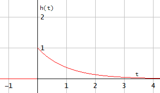
In this presentation I will not use units, for my own convenience. The impulse response $h$ of a resistor-capacitor (RC) filter, as function of continuous time $t$, is of form:

$$h(t) = \begin{cases}0&\text{if }t<0,\\\displaystyle a e^{-at}&\text{if }t\ge0,\end{cases}\tag{1}$$

enter image description here
Figure 1. RC-filter impulse response (Eq. 1), with decay parameter $a = 1$.

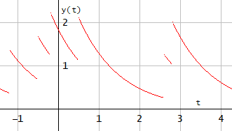
where $a$ is a positive constant that determines the decay rate. If this is convolved with a realization of a Poisson process with $K$ Dirac impulse events at times $p_k$, $0 < k \le K$, then we get the signal $y$ of which you can find some literature under the keyword filtered Poisson process:

$$y(t) = \sum_k^{K-1}h\left(t-p_k\right)\tag{2}$$

enter image description here
Figure 2. A realization of an RC-filtered Poisson process (Eq. 2), with $a = 1$.

We can set up a sample point at time $t_n$. If we know the signal value $y(t_n)$ at that point, then we can forget the events at or before that time and still reconstruct $y(t)$ at later times $t \ge t_n$:

$$y(t) = y(t_n)\,e^{-a(t-t_n)} + \sum_{k=0}^{K-1}\begin{cases}0&\text{if }p_k \le t_n,\\h(t-p_k)&\text{if }p_k > t_n,\end{cases}\quad t \ge t_n,\tag{3}$$

or in a less formal short-hand notation:

$$y(t) = y(t_n)\,e^{-a(t-t_n)} + \sum_{k,\,t_n < p_k}h(t-p_k), \quad t \ge t_n.\tag{4}$$

This is a property unique to the one-sided exponential function $h(t)$. The effect of an event at time $p_k$ is already included in $y(p_k)$ with the way Eq. 1 is currently defined. We can make explicit also that because the impulse response is causal, the events happening after time $t$ do not affect $y(t)$:

$$y(t) = y(t_n)\,e^{-a(t-t_n)} + \sum_{k,\,t_n<p_k\le t}h(t-p_k), \quad t \ge t_n.\tag{5}$$

You can do non-uniform sampling at the event times by setting $t_k = p_k$, or uniform sampling with sampling period $\Delta t$ by setting $t_n = t_0 + n\,\Delta t$. In your data structure you'd just store $t_n$ (no need in case of uniform sampling) and $y(t_n)$. Python example:

import numpy as np
import bisect
import matplotlib.pyplot as plt

sim_length = 10  # Simulation length
rate = 100  # Event rate per time unit
a = 1  # Filter decay constant

K = np.random.poisson(rate*sim_length)  # Number of events
N = K + 1  # Number of samples. Always have one sample at simulation start
ty = np.empty(N, dtype = [('time', float), ('value', float)])  # Sample times t and signal values y
ty['time'][0] = 0 
ty['value'][0] = 0  # Start signal at value 0
ty['time'][1:] = np.random.uniform(0, sim_length, K)  # Event times
ty[1:].sort(order='time')  # Sort events by time
for k in range(K):  # Sample signal at event times
    ty['value'][1 + k] = ty['value'][k]*np.exp(-a*(ty['time'][1 + k] - ty['time'][k])) + a

def sample_y(ty, t):  # Sample signal at arbitrary time t
    k = bisect.bisect(ty['time'], t) - 1     
    return ty['value'][k]*np.exp(-a*(t-ty['time'][k]))

# Create a time series of the RC-filtered Poisson process
t = np.arange(0, sim_length, 1/10000)  # Delta t = 1/10000
y = np.zeros(t.size)
for k in range(t.size):
    y[k] = sample_y(ty, t[k])

# Plot
plt.plot(t, y)
plt.xlabel('t')
plt.ylabel('y(t)')
plt.show()

enter image description here
Figure 3. RC-filtered Poisson process plotted by the above Python script.

enter image description here
Figure 4. RC-filtered Poisson process reparameterized with rate = 1 and a = 10.

$\endgroup$
1
  • $\begingroup$ Thanks for the reply, I have been trying to digest your answer but I'm having hard time putting it into a practical perspective, maybe some simple python code would go a long way! $\endgroup$
    – Knyq
    Commented May 11, 2019 at 2:01
3
$\begingroup$

This is an excellent series of questions, so I will have a go at part of it! I will start with an example from Verdeyen’s book (J. T. Verdeyen, Laser Electronics, Prentice-Hall, Inc., Englewood Cliffs, NJ, ©1981, Chapter 14). Assume $\lambda$ = 500 nm, quantum efficiency = 0.15, photomultiplier (PMT) gain = 1.68x$10^7$, transimpedance = 1 k$\Omega$ and RC= 100 $\mu$s. Assume $\Delta$t = 1 $\mu$s and the output of the RC LPF is sampled at the end of every 100 $\mu$s interval. Start at the bottom: assume an average of 2 photons/$\mu$s arrive at the PMT’s photocathode. Then the average incident optical power is 0.795 pW, the average photocurrent is 806 nA and the TIA’s average output voltage is 0.806 mV. The first figure below shows the Mueller calculus simulation models, with the above assumptions. (It is deliberately simple, for present purposes, but can be made much more complicated and realistic if desired.)

Mueller calculus simulation models

The light source produces Stokes vectors at the rate of 1/$\mu$s, and the intensity is proportional to the number of photons in that $\mu$s interval. The detector and transimpedance preamplifier (TIA) converts the incident light intensities to photocurrents and then to voltages. The FFT PSD block shows (second figure) that the noise is white.
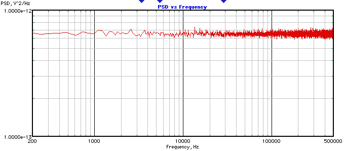
PSD of the TIA

Then the RC LPF filters the TIA’s outputs and its outputs are sampled every 100 $\mu$s and also processed to yield a PSD (third figure). The TIA's PSD is the average of 1000 8k FFT PSDs, the RC LPF's PSD is the average of just 100 8k FFT PSDs (Fig. 1B shows the data collection only, but not the separate FFT PSD processing), and they are all unilateral and mean-subtracted.
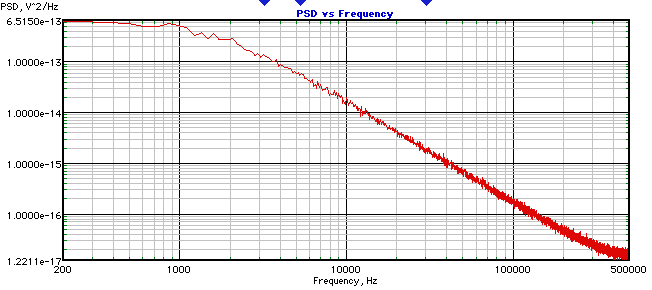
PSD of the RC LPF

The fourth figure shows the raw TIA output (green), the RC LPF output (cyan) and the sampled RC LPF output (red). The quantization at low photon flux is clearly shown in the TIA output

Outputs for m = 2

Increasing the photon flux to 20 photons/$\mu$s gives the results in the fifth figure. Now the quantization is not so bad and the signal-to-noise ratio is higher, as expected. Increasing the photon flux further makes it reasonable to replace the Poisson distribution with its ‘envelope’ Gaussian distribution (not shown here). Hope this helps a bit: there is FAR more that can be said!

Outputs for m = 20

Note: I have corrected the first three figures to be consistent with the 'sample calculation' values given several paragraphs below. I will go through and update everything as needed or necessary!

The software I use is ExtendSim (commercial simulation software from Imagine That, Inc.), augmented with my free LightStone libraries of blocks (with full commented source code for all blocks). It is easy to construct time-series after the S&H and find the variance: I have been playing with just that since I saw your comment. Now for the specific question you ask, if photon flux is constant, at 2 photons/$\mu$s (= 20 photons/10$\mu$s), then the distinction is in the measurement interval, $\tau$. For the former, $\tau$ = 1 $\mu$s, so the mean number of photons in the measurement interval, m, is 2. For the latter, $\tau$ = 10 $\mu$s, m = 20 = 2 photons/$\mu$s x 10 $\mu$s. If the simulation step size, $\Delta$t, is constant at 1 $\mu$s, then the average signal magnitude in the larger $\tau$ will be 20/2 times larger than in the smaller $\tau$. The unilateral PSD will also be directly proportional to m, so it will be 10 times larger as well. Hence the variance at the output of the RC LPF will be 10 times larger (to the extent that the digital RC LPF ‘honors’ the analog RC LPF’s 1/4RC noise bandwidth), so the standard deviation will be $10^{1/2}$ times larger. So the SNR, as signal magnitude/noise standard deviation, is $10^{1/2}$ times larger, as expected for shot noise. By the way, in my field, SNRs are not usually done as signal power/noise power.

I ran the sims for the cases of m = 2 (with $\Delta$t = 1 $\mu$s) and m = 20 (with $\Delta$t = 1 $\mu$s and also with $\Delta$t = 10 $\mu$s), sampling (via the S&H) every 100 $\mu$s to get time-series. Each sim ran from 0 to 0.1 s and the S&H was sampled every 100 $\mu$s. I collected 1000 values for each series and discarded the data for the first 500 $\mu$s, because an RC LPF settles to 1% in 4.605 time constants. So each series is 995 S&H values, collected at 100 $\mu$s intervals.

Results summary: For m = 2, $\Delta$t = 1 $\mu$s, and $\tau$ = 1 $\mu$s, the average = 0.000807 V and standard deviation = 0.0000399 V. For m = 20, $\Delta$t = 10 $\mu$s, and $\tau$ = 10 $\mu$s, the average = 0.00808 V and the standard deviation = 0.000406 V. For m = 20, $\Delta$t = 1 $\mu$s, and $\tau$ = 10 $\mu$s, the average = 0.00807 V and the standard deviation = 0.000130 V. Note that 0.000130 V/0.0000399 V = 3.258, which is approximately $10^{1/2}$. N.B.: the ‘volt' units are fictitious, of course, since this is just a simulation!

Sample calculation: The unilateral PSD, at the output of the TIA, is m photons x 2 x $(0.0004037 V/photon)^2$ x $\Delta$t. For m = 2, this yields 6.52 x $10^{-13}$ $V^2$/Hz. Then the variance at the output of the digital RC LPF (if the noise bandwidth was actually 1/4RC), would be 6.52 x $10^{-13}$ $V^2$/Hz x 1 x 1/400 $\mu$s = 1.63 x $10^{-9}$ $V^2$, so the standard deviation would be 4.04 x $10^{-5}$. This is close to the above 3.99 x $10^{-5}$ V. Hope this helps.

Added 5/14/2019: For m = 2, $\Delta$t = 1 $\mu$s, and $\tau$ = 1 $\mu$s, I collected 100 files of 8k each, neglecting the first 1 ms (i.e., 10 RC times constants, to generously allow for settling of the RC LPF). I did this for 10 kHz sampling of the S&H and again for 100 kHz sampling of the S&H. For the 10 kHz sampling, the average variance of the 100 8k time series was 1.628 x $10^{-9}$ V and the PSD is shown below:

PSD of S&H at 10 kHzsampling

From the first PSD, the rms value was 4.035 x $10^{-5}$ V. This is the same, to 4 digits, as the square root of the variance.

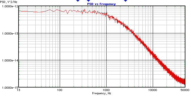
For the 100 kHz sampling, the average variance of the 100 8k time series was 1.632 x $10^{-9}$ V and the PSD is shown below:
PSD of S&H at 100 kHz sampling

From the second PSD, the rms value was 4.039 x $10^{-5}$ V. The square root of the variance was 4.040 x $10^{-5}$ V.

$\endgroup$
9
  • $\begingroup$ Thank you so much for this! A lot to process! May I ask what software did you use for the simulation? Im very interested in reproducing your simulations and try my variations too. Is it possible to construct a time-series after the SH and evaluate the noise power (variance) of it? Also, here you change the light level but what happens if the light level remains constant but the sampling time is elongated (eg you use 2 ph/us and 20 ph/us, I would use 2ph/us and 20ph/10us) and then these two systems go through the same chain. Is there a change in the time-series variance because of this? $\endgroup$
    – Knyq
    Commented May 11, 2019 at 16:08
  • $\begingroup$ In response to Knyq's comment, I have added some germane material. $\endgroup$
    – Ed V
    Commented May 12, 2019 at 0:47
  • $\begingroup$ Thanks again Ed V! I was expecting the simulation step size $\Delta t$ to increase with the measurement interval $\tau$, how do you extend the measurement signal with the additional samples now that your measurement interval is 10 times the simulation interval? A couple more questions to come once I digested the results! Thanks! $\endgroup$
    – Knyq
    Commented May 12, 2019 at 7:36
  • $\begingroup$ I actually ran the m = 2 case with two different values of the sim step size, so I have added this to the answer. It is very easy to go too fast and make silly omissions and mistakes! P.s. Can anyone tell me what the little gray flags mean? Have I violated some site rule or whatever? If so, I apologize! $\endgroup$
    – Ed V
    Commented May 12, 2019 at 13:02
  • $\begingroup$ Ed V, one more question. For the case $Delta t =1us$ Could you post the PSD plot of the SH (and variance of related time series) if you change SH sampling frequency to 1sample/10us? In short I wanna see the effect of oversampling of the SH. $\endgroup$
    – Knyq
    Commented May 14, 2019 at 5:10

Your Answer

By clicking “Post Your Answer”, you agree to our terms of service and acknowledge you have read our privacy policy.

Not the answer you're looking for? Browse other questions tagged or ask your own question.