Extended Kalman Filter (EKF) for Non Linear (Coordinate Conversion - Polar to Cartesian) Measurements and Linear Predictions

Question

I'm new to Kalman filtering and state estimation and I'd like some guidance on EKFs.

Currently, I'm trying to use a linear prediction model coupled with nonlinear measurements to estimate the state of an object. My state vector ($\bar{x}$) is:

\begin{bmatrix}x\\y\\v_x\\v_y\end{bmatrix}

and my state model is (with no process noise ($W_k$) or process noise covariance ($Q_k$)): $$ \bar{x}_{k_p} = A\bar{x}_{k-1} \ + B\begin{bmatrix} a_x \\ a_y \end{bmatrix} $$

$$ P_{k_p} = AP_{k-1}A^T $$ where $$ A = \begin{bmatrix} 1 & 0 & \Delta T & 0 \\ 0 & 1 & 0 & \Delta T \\ 0 & 0 & 1 & 0 \\ 0 & 0 & 0 & 1 \end{bmatrix} $$ and $$ B = \begin{bmatrix} \frac{1}{2}\Delta T^2 & 0 \\ 0 & \frac{1}{2}\Delta T^2 \\ \Delta T & 0 \\ 0 & \Delta T\end{bmatrix} $$

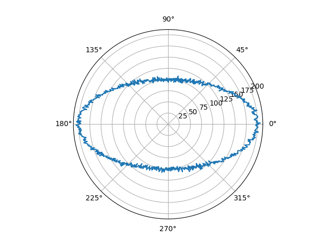
I have simulated some measurement data with Gaussian noise. The measurements are outputted as $\begin{bmatrix}r\\\theta\end{bmatrix}$, and this is the graph of the generated data:

To account for the polar coordinates, I was going to use a function $h(z)$ that transformed from polar to cartesian coordinates in my state update equation $\bar{x}_k = \bar{x}_{k_p} \ + K_k(h(\bar{z}_k)-\bar{x}_{k_p})$? This seemed like the simple thing to do, but this post does say that if I did so, my filter wouldn't work as the polar to cartesian transform isn't a linear transform.

To resolve this, I want to use an EKF to linearize the measurements, and after reading a few articles online, my gain calculation and update step are as follows:

$$ K_k = P_kJ(\bar{z}_k)^T \ (J(\bar{z}_k)P_kJ(\bar{z}_k)^T + R)^{-1} $$

$$ \bar{x}_k = \bar{x}_{k_p} \ + K_k(Z_k - H\bar{x}_{k_p}) $$

$$ P_k = (I - K_k J(\bar{z}_k))P_{k_p} $$

where $K_k$ is the Kalman gain, $\bar{z}_k$ is the measurement vector outputted by the sensor, and $J(\bar{z}_k)$ is a Jacobian to linearize the polar coordinate measurements. These are all at time $k$. In addition, my prediction equations are the same linear equations as shown above.

I used $x = r \cos(\theta)$ and $y = r \sin(\theta)$ to derive the following Jacobian: $$ J(r,\theta) = \begin{bmatrix} \frac{\partial x}{\partial r} & \frac{\partial x}{\partial \theta} \\ \frac{\partial y}{\partial r} & \frac{\partial y}{\partial \theta} \\ \frac{\partial v_x}{\partial r} & \frac{\partial v_x}{\partial \theta} \\ \frac{\partial v_y}{\partial r} & \frac{\partial v_y}{\partial \theta} \\ \end{bmatrix} = \begin{bmatrix} \cos(\theta) & -r\sin(\theta) \\ \sin(\theta) & r\cos(\theta) \\ 0 & 0 \\ 0 & 0 \end{bmatrix} $$

Would this Jacobian and model be the correct way to go about my problem? Thanks for your help!

P.S. I'm super new to this so if some of my lingo is wrong or weird, if I'm missing something or something makes no sense, or if you have some tips to better my understanding, please let me know. Thanks!

EDIT: I converted the polar values to the cartesian plane with $x = r\cos(\theta)$ and $y=r\sin(\theta)$, and then graphed the $x$ and 4y$ values. This is the result:

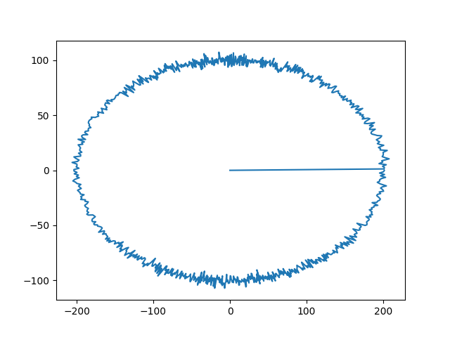
Obviously, something seems to be working, but I don't know/understand why, especially if the transform isn't linear. If someone could help my understanding of this as well, I'd truly appreciate it.

Answer 1

Update

If I understood your model, you have a model of Constant Velocity in 2D (Cartesian Coordinate System).
While your measurement are in Polar Coordinate System.

Pay attention that your measurement function is:

$$ h \left( x, y, {v}_{x}, {v}_{y} \right) = \begin{bmatrix} \sqrt{ {x}^{2} + {y}^{2} } \\ {\tan}^{-1} \left( \frac{y}{x} \right ) \end{bmatrix} $$

Hence you Jacobian becomes:

$$\begin{aligned} {J}_{h} \left( x, y, {v}_{x}, {v}_{y} \right) & = \begin{bmatrix} \frac{\partial \sqrt{ {x}^{2} + {y}^{2} } }{\partial x} & \frac{\partial \sqrt{ {x}^{2} + {y}^{2} } }{\partial y} & \frac{\partial \sqrt{ {x}^{2} + {y}^{2} } }{\partial {v}_{x}} & \frac{\partial \sqrt{ {x}^{2} + {y}^{2} } }{\partial {v}_{y}} \\ \frac{\partial {\tan}^{-1} \left( \frac{y}{x} \right ) }{\partial x} & \frac{\partial {\tan}^{-1} \left( \frac{y}{x} \right ) }{\partial y} & \frac{\partial {\tan}^{-1} \left( \frac{y}{x} \right ) }{\partial {v}_{x}} & \frac{\partial {\tan}^{-1} \left( \frac{y}{x} \right ) }{\partial {v}_{y}} \end{bmatrix} \\ & = \begin{bmatrix} \frac{x}{ \sqrt{ {x}^{2} + {y}^{2} } } & \frac{y}{ \sqrt{ {x}^{2} + {y}^{2} } } & 0 & 0 \\ -\frac{y}{{x}^{2} + {y}^{2}} & \frac{x}{{x}^{2} + {y}^{2}} & 0 & 0 \end{bmatrix} \end{aligned}$$

The function of the measurement is the one connecting your state vector into the measurement and not the other way around.

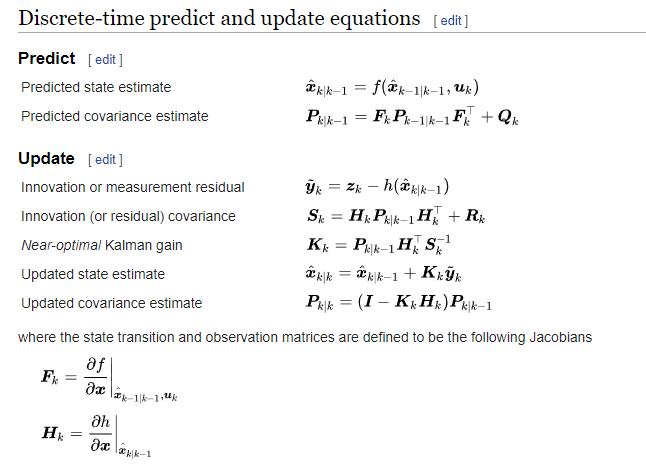
Let's look on Wikipedia EKF Model:

In you case $ F $ is constant is the model is linear.
What's in Wikipedia called $ H $ is the $ J $ I derived above.
Dimension wise, all is perfectly defined.

Implementation

I implemented a general Kalman Filter Iteration with support for Extended Kalman Filter (With option for Numeric Calculation of the Jacobian).
I also added option to Unsecented Kalman Filter (UKF) Iteration, so you will be able to compare.

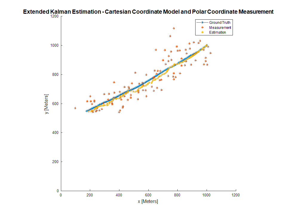
Here is a result in with the same model as yours:

The full code is available on my StackExchange Signal Processing Q51386 GitHub Repository (Look at the SignalProcessing\Q51386 folder).

24/08/2018: I added UKF implementation which is pretty general so you could use it in various models.

Original Answer

Converting coordinate system is the main reason the Extended Kalman Filter was invented.

Let me give you a tip, it doesn't work well in those cases.
If you use Non Linear Transformation use something that will both make things easier and better (Yea, usually it doesn't work like that, but in this case it does) - Use the Unscented Kalman Filter (UKF) which is based on the Unscented Transform.
Once you utilize that there is no need to derive the Jacobian.
All needed is to apply the non linear function $ n $ times (On each Sigma Point).

It is easy to see that linearization doesn't work well for propagating the mean and the covariance in many (Most) cases.
The UKF directly approximate the calculation of the integration of the non linear function which calculates the mean and covariance.

It will make things easier as you'll be able to skip the linearization step and only know the coordinate transformation function.

In modern tracking we usually stay away from EKF and utilize methods which better approximate the integrals of the first 2 moments propagation.
The most common ones are the UKF and GHKF (Those are called Sigma Points Kalman filters).
Their generalization is the Particle Filter which in most cases is over kill.

Update
Have a look at EKF / UKF Maneuvering Target Tracking using Coordinated Turn Models with Polar/Cartesian Velocity.

From their conclusion:

We have shown a range of coordinated turn (CT) models using either Cartesian or polar velocity and how to use them in a Kalman filtering framework for maneuvering target tracking. The results of the conducted simulation study are in favor of polar velocity. This confirms the results of the previous study [11] and extends it to the case of varying target speed. For polar CT models, the performance in terms of position RMSE of the predicted state appears to be comparable for EKF and UKF. As the UKF does not require the derivation and implementation of Jacobians it might be more straightforward to implement. The RMSE provided by the Cartesian velocity EKF and UKF turned out slightly worse. Interestingly, the sensitivity of the RMSE with respect to the noise parameters was decreased by using EKF2 and UKF in the Cartesian case. This, in addition to the simpler implementation and lower computational cost of UKF over EKF2 results in a recommendation for UKF if Cartesian CT models are preferred.

Basically telling you, don't bother with Jacobians, just use the simpler UKF.

Another comparison is made at Implementation of the Unscented Kalman Filter and a simple Augmentation System for GNSS SDR receivers with:

As can be seen, UKF implementation does not require linearization (state transition function and measurements functions are directly applied to sigma points) and it can also work in presence of discontinuities. The prediction only consists of linear algebra operations. All such advantages are fundamental for minimizing computational load in an SDR implementation.

While the classical Kalman Filter implies the propagation of n components for the state vector and n2 /2+n/2 components for the Covariance matrix, the UKF requires the propagation of 2n+1 sigma points only.

Furthermore, UKF is more insensitive to initial conditions with respect to EKF. It has been demonstrated that UKF rapidly converge also in presence of an initial position error of several Kilometers.

Answer 2

UPDATE

It looks like we are all stumbling forward

This section is wrong, and I appreciate being corrected.

First your Jacobian is incorrect for the polar to cartesian transform,  from

https://en.wikipedia.org/wiki/Jacobian_matrix_and_determinant 

$$
\begin{align}
x &= r \cos \varphi ; \\
y &= r \sin \varphi .
\end{align}$$

$$\mathbf J_{\mathbf F}(r, \varphi) = \begin{bmatrix}
  \dfrac{\partial x}{\partial r} & \dfrac{\partial x}{\partial\varphi}\\[1em]
  \dfrac{\partial y}{\partial r} & \dfrac{\partial y}{\partial\varphi} \end{bmatrix}
= \begin{bmatrix}
  \cos\varphi & - r\sin \varphi \\
  \sin\varphi &   r\cos \varphi \end{bmatrix}
$$

$R^2 \rightarrow R^2$ Jacobians are square.

the stumble forward part

Unless your measurement angles are limited to the first and second quadrant, I believe the measurement equation should be:

$$ g\left((r=\sqrt{x^2+y^2},\theta=\text{atan2}(y,x)\right)=\left| \begin{array}{c} r \\ \theta \end{array}\right|_{r=\sqrt{x^2+y^2} \\ \theta=\text{atan2}(y,x)} $$

According to https://en.wikipedia.org/wiki/Atan2 the partial derivatives are the same as for $\text{atan}(y/x)$ so the Jacobian that @Royi is correct, but the measurement equation he gives is not correct for $-\pi\le \theta \le \pi$.

End Update

The post says the filter might not work. This is a situation where you need to experiment and there are no hard and fast rules. There are Extended Kalman Filters as opposed to is an EKF. There are filters that are first order and filters that are second order. There are iterated filters.

One difficulty with using nonlinearities directly in the state variable evolution is the difficulty of the nonlinear integration update to propagate the mean. Most old books will try to modify Euler Integration by using terms of the Taylor Series. You can also use an ODE solver like Runge Kutta integration.

The second difficulty is propagation of variance. One can use Taylor Series terms or you can use a UKF or particle filter by estimating the spread by numerical integration. For the UKF, quadrature or importance sampling for the particle filter.

In mixed systems where just the measurement or just the state is nonlinear, you can treat the linear part as linear which is known as Rao Blackwellization .

The KF/EKF doesn’t require process noise but you have a kinematic state variable motion model which is kind of dull without process noise. Measurement noise is required for the filter to work. If you don’t have measurement noise you use a state observer and don’t need a filter.

There are many papers on the kind of problem you describe. Some with a nonlinear measurement model and some with a nonlinear state model. Using inverse range as a coordinate system is very common, particularly in bearing only measurement cases.

The book Samuel S. Blackman - Multiple-target Tracking with Radar Applications covers coordinate systems and transformation issues in detail. The book is expensive but should be available in a good library. There are many ways to approach the problem.

An EKF can be much more than a linearization. A UKF actually uses the nonlinearity directly and so can a EKF with ODE integration.

It should be pointed out that step size has an effect.

IMHO, It should be called a smorgasbord Kalman Filter.

To answer your question, using the nonlinearity directly to propagate the mean ( predicted measurement) is often OK. On the measurement side there isn’t an integration. The covariance update is the tricky part. Linearization is the most common approach. The UKF uses the nonlinearity directly so it would be odd to say it was a “bad idea “

some edits:

Even in the linear state, linear measurement scenario, kinematic tracking state variable models don't include aerodynamic drag which is approximated by a term proportional to the velocity squared. Process noise covers modeling errors as well as the perturbative random forces that a body may encounter.

Process noise is also important because it controls the relative significance of a measurement and weighs the state variable evolution to either the prediction or the measurement. Without process noise a filter can't follow deviations from the state model. Your filter can track. There is a technique called Interacting Multiple Models (IMM) that is suitable to large deviations in the state model but I'm not going to mention it further.