0
$\begingroup$

I am trying to implement GCC-PHAT in python.

The approach is similar to the following two links: link1 and link2

It seems the only difference between GCC-PHAT and normal cross-correlation using FFT is the division by the magnitude.

Here is my code:

import numpy as np
import matplotlib.pyplot as plt
from scipy.fftpack import rfft, irfft, fftfreq, fft, ifft

def xcorr_freq(s1,s2):
    pad1 = np.zeros(len(s1))
    pad2 = np.zeros(len(s2))
    s1 = np.hstack([s1,pad1])
    s2 = np.hstack([pad2,s2])
    f_s1 = fft(s1)
    f_s2 = fft(s2)
    f_s2c = np.conj(f_s2)
    f_s = f_s1 * f_s2c
    denom = abs(f_s)
    denom[denom < 1e-6] = 1e-6
    f_s = f_s / denom  # This line is the only difference between GCC-PHAT and normal cross correlation
    return np.abs(ifft(f_s))[1:]

I have checked by commenting out fs = fs / denom The function produces the same result as normal cross correlation for a wide band signal.

Here is a sample test code which shows the GCC-PHAT code above performs worse than normal cross-correlation:

LENG = 500
a = np.array(np.random.rand(LENG))
b = np.array(np.random.rand(LENG))
plt.plot(xcorr_freq(a,b))
plt.figure()
plt.plot(np.correlate(s1,s2,'full'))

Here is the result with GCC-PHAT:
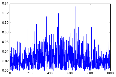
enter image description here

Here is the result with normal cross-correlation:
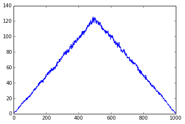
enter image description here

Since GCC-PHAT should give better cross-correlation performance for wide band signal, I know there is something wrong with my code. Any help is very appreciated!

$\endgroup$
1
  • $\begingroup$ Concerning your second code fragment: how did you compute s1 and s2? I think that with np.correlate you compute something totally different from what you get with xcorr_freq. Your code for xcorr_freq looks OK. $\endgroup$
    – Matt L.
    Commented Sep 4, 2014 at 9:07

1 Answer 1

1
$\begingroup$

Yep, as Matt L. state in their comment your code is correct... As can be seen in the figures you've provided your GCC PhaT works quite well!

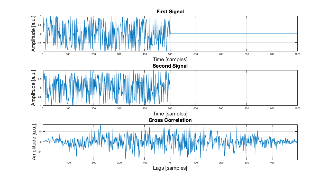
If you have a look in the literature, you'll realise that the cross-correlation of two independent random vectors, like your vectors, doesn't peak somewhere, since they are "purely" random and their samples are not correlated in any way. Below you can see the results I get from "simple" cross correlation implemented in the frequency domain, like you did. The random vectors are drawn from a uniform distribution.

Cross correlation of two random vectors (uniform distribution)

According to its documentation np.correlate does perform correlation, albeit in the time domain. Now, you get "unexpectedly" different results because you have different expectations. This means that the results you get should be what they are depending on what the signals s1 and s2 are. In the FFT version of your correlation (not sure if you still have the "PhaT version" commented or not) you use a and b while you use s1 and s2 for your time domain version. Most probably the two pairs of variables do not hold the same vectors.

Additional info

Although your code for GCC PhaT seems to be OK (haven't tested it but all necessary steps seem to be present) there is some "better" approach to calculate the "PhaT filter". According to the filters formula

$$ y_{PhaT} \left( l \right) = \mathcal{IFFT} \left\{ \frac{G_{x y}}{\left| G_{x y} \right|} \right\}$$

where $y_{PhaT}$ is the PhaT cross correlation function, $l$ is the lag index (the free variable of the function), $\mathcal{IFFT}$ denotes the Inverse Fourier Transform, $G_{x y}$ the cross spectrum and $\left| ~ \cdot ~ \right|$ denotes magnitude.

The idea is that you only retain the phase information of the function, since time is entirely encoded in the phase. Thus, instead of dividing by the magnitude to, correctly in the mathematical sense, replicate the formula, you can just use the phase of the cross spectrum, which you can get with np.angle(f_s). This way you avoid division with zero, or the need to clamp the values of the magnitude to avoid numerical overflows, or "explosions". Consequently, you can calculate the GCC PhaT functions as ifft(np.exp(1j * np.angle(f_s))).

As a final remark, please note that if there's any numerical errors resulting in imaginary values in the time-domain (after the inverse transform) you should get the real part of it and not the absolute value/magnitude.

$\endgroup$

Your Answer

By clicking “Post Your Answer”, you agree to our terms of service and acknowledge you have read our privacy policy.

Not the answer you're looking for? Browse other questions tagged or ask your own question.