update with full fix
Source Link
geometrikal
  • 3.6k
  • 16
  • 27

I wrote some MATLAB code to locate the angles and mean separation between lines.


close all
I = imread('testimage'testt.jpg');
I = rgb2gray(I);
I = I(2:end-1,:);

% Radon transform
R = radon(I,0:179);
imagesc(R); colormap gray(256); pause;

% Chop offRadon outtransform of rangesmoothed partsimage
chopRg = sizeradon(R,1) - sizeimgaussian(I,1);
chop = ceil(chop/2);
R = R(chop+1:end-chop,0:179);
imagesc(RRg); colormap gray(256); pause;

% GaussianTake smoothingit away
RgRf = imgaussian(R,2); - Rg;
imagesc(RgRf); colormap gray(256); pause;

% TakeChop itoff awayout of range parts
Rfchop = Rsize(Rf,1) - Rg;size(I,1);
chop = ceil(chop/2);
Rf = Rf(chop+1:end-chop,:);
imagesc(Rf); colormap gray(256); pause;

% Negative lines - threshold
Rf(Rf > 0) = 0; 
imagesc(Rf); colormap gray(256); pause;

% Plot sum - peaks are angles
Rp = sum(abs(Rf));
plot(Rp);

% Get the peaks sep by at least 15 deg
[p,a] = findpeaks(Rp,'minpeakdistance',15,'sortstr','descend');
hold on;
scatter(a,p,'r*');
hold off;
pause;

% Iterate through peaks and find fequencies
for j = 1:numel(a)
    % Get subsection of Radon transform around angle and transpose
    vstart = max([a(j)-10,1]);
    vend = min([a(j)+10,size(Rf,2)]);
    Rsub = Rf(:,vstart:vend).';
    imagesc(Rsub); colormap gray(256); pause;
    RsubP = sum(abs(Rsub));
    plot(RsubP); pause;
    
    % Find peak correlation with a bit of smoothing
    xp = xcorr(imgaussian(RsubP,2),imgaussian(RsubP,2));
    plot(xp); pause;
    [rp,rl] = findpeaks(xp,'sortstr','descend');
    wave(j) = abs(rl(1) - rl(2));
    disp(['Angle: ' num2str(a(j))]);
    disp(['Wavelength: ' num2str(wave(j))]);
    disp(['Strength: ' num2str(p(j))]);
    pause;
end

Still have to work out how to get the frequencies by this method though.and

Angle: 73
Wavelength: 16
Strength: 12401.356

Angle: 92
Wavelength: 54
Strength: 9442.2545

Angle: 175
Wavelength: 33
Strength: 9030.1877

I wrote some MATLAB code to locate the angles.


close all
I = imread('testimage.jpg');
I = rgb2gray(I);
I = I(2:end-1,:);

% Radon transform
R = radon(I,0:179);
imagesc(R); colormap gray(256); pause;

% Chop off out of range parts
chop = size(R,1) - size(I,1);
chop = ceil(chop/2);
R = R(chop+1:end-chop,:);
imagesc(R); colormap gray(256); pause;

% Gaussian smoothing
Rg = imgaussian(R,2);
imagesc(Rg); colormap gray(256); pause;

% Take it away
Rf = R - Rg;
imagesc(Rf); colormap gray(256); pause;

% Negative lines - threshold
Rf(Rf > 0) = 0; 
imagesc(Rf); colormap gray(256); pause;

% Plot sum - peaks are angles
Rp = sum(abs(Rf));
plot(Rp);

% Get the peaks sep by at least 15 deg
[p,a] = findpeaks(Rp,'minpeakdistance',15,'sortstr','descend');
hold on;
scatter(a,p,'r*');
hold off;

Still have to work out how to get the frequencies by this method though.

I wrote some MATLAB code to locate the angles and mean separation between lines.


close all
I = imread('testt.jpg');
I = rgb2gray(I);
I = I(2:end-1,:);

% Radon transform
R = radon(I,0:179);
imagesc(R); colormap gray(256); pause;

% Radon transform of smoothed image
Rg = radon(imgaussian(I,2),0:179);
imagesc(Rg); colormap gray(256); pause;

% Take it away
Rf = R - Rg;
imagesc(Rf); colormap gray(256); pause;

% Chop off out of range parts
chop = size(Rf,1) - size(I,1);
chop = ceil(chop/2);
Rf = Rf(chop+1:end-chop,:);
imagesc(Rf); colormap gray(256); pause;

% Negative lines - threshold
Rf(Rf > 0) = 0; 
imagesc(Rf); colormap gray(256); pause;

% Plot sum - peaks are angles
Rp = sum(abs(Rf));
plot(Rp);

% Get the peaks sep by at least 15 deg
[p,a] = findpeaks(Rp,'minpeakdistance',15,'sortstr','descend');
hold on;
scatter(a,p,'r*');
hold off;
pause;

% Iterate through peaks and find fequencies
for j = 1:numel(a)
    % Get subsection of Radon transform around angle and transpose
    vstart = max([a(j)-10,1]);
    vend = min([a(j)+10,size(Rf,2)]);
    Rsub = Rf(:,vstart:vend).';
    imagesc(Rsub); colormap gray(256); pause;
    RsubP = sum(abs(Rsub));
    plot(RsubP); pause;
    
    % Find peak correlation with a bit of smoothing
    xp = xcorr(imgaussian(RsubP,2),imgaussian(RsubP,2));
    plot(xp); pause;
    [rp,rl] = findpeaks(xp,'sortstr','descend');
    wave(j) = abs(rl(1) - rl(2));
    disp(['Angle: ' num2str(a(j))]);
    disp(['Wavelength: ' num2str(wave(j))]);
    disp(['Strength: ' num2str(p(j))]);
    pause;
end

and

Angle: 73
Wavelength: 16
Strength: 12401.356

Angle: 92
Wavelength: 54
Strength: 9442.2545

Angle: 175
Wavelength: 33
Strength: 9030.1877
big update with code
Source Link
geometrikal
  • 3.6k
  • 16
  • 27

Another approach might be to perform the Radon / Hough transform first, then detect the points.

e.g. R = radon(I,0:179) in MATLAB.

It gives this image:

enter image description here

The x-axis is angle (0-180 deg) and the y-axis is distance from the centre. Each local minimum represents a line. It shows 6 lines ~75 degrees, 2 around 90 degrees, and 3 around 170 degrees. (This is MATLAB angles which go clockwise from x-axis because the y-coords are upside down)

Edit: Forgot Radon and Hough transforms were roughly the same.

Update:

I wrote some MATLAB code to locate the angles.


close all
I = imread('testimage.jpg');
I = rgb2gray(I);
I = I(2:end-1,:);

% Radon transform
R = radon(I,0:179);
imagesc(R); colormap gray(256); pause;

% Chop off out of range parts
chop = size(R,1) - size(I,1);
chop = ceil(chop/2);
R = R(chop+1:end-chop,:);
imagesc(R); colormap gray(256); pause;

% Gaussian smoothing
Rg = imgaussian(R,2);
imagesc(Rg); colormap gray(256); pause;

% Take it away
Rf = R - Rg;
imagesc(Rf); colormap gray(256); pause;

% Negative lines - threshold
Rf(Rf > 0) = 0; 
imagesc(Rf); colormap gray(256); pause;

% Plot sum - peaks are angles
Rp = sum(abs(Rf));
plot(Rp);

% Get the peaks sep by at least 15 deg
[p,a] = findpeaks(Rp,'minpeakdistance',15,'sortstr','descend');
hold on;
scatter(a,p,'r*');
hold off;

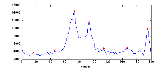
which results in: (red * are possible angles)

enter image description here

Still have to work out how to get the frequencies by this method though.

Another approach might be to perform the Radon / Hough transform first, then detect the points.

e.g. R = radon(I,0:179) in MATLAB.

It gives this image:

enter image description here

The x-axis is angle (0-180 deg) and the y-axis is distance from the centre. Each local minimum represents a line. It shows 6 lines ~75 degrees, 2 around 90 degrees, and 3 around 170 degrees. (This is MATLAB angles which go clockwise from x-axis because the y-coords are upside down)

Edit: Forgot Radon and Hough transforms were roughly the same.

Update:

I wrote some MATLAB code to locate the angles.


close all
I = imread('testimage.jpg');
I = rgb2gray(I);
I = I(2:end-1,:);

% Radon transform
R = radon(I,0:179);
imagesc(R); colormap gray(256); pause;

% Chop off out of range parts
chop = size(R,1) - size(I,1);
chop = ceil(chop/2);
R = R(chop+1:end-chop,:);
imagesc(R); colormap gray(256); pause;

% Gaussian smoothing
Rg = imgaussian(R,2);
imagesc(Rg); colormap gray(256); pause;

% Take it away
Rf = R - Rg;
imagesc(Rf); colormap gray(256); pause;

% Negative lines - threshold
Rf(Rf > 0) = 0; 
imagesc(Rf); colormap gray(256); pause;

% Plot sum - peaks are angles
Rp = sum(abs(Rf));
plot(Rp);

% Get the peaks sep by at least 15 deg
[p,a] = findpeaks(Rp,'minpeakdistance',15,'sortstr','descend');
hold on;
scatter(a,p,'r*');
hold off;

which results in: (red * are possible angles)

enter image description here

Still have to work out how to get the frequencies by this method though.

added 103 characters in body
Source Link
geometrikal
  • 3.6k
  • 16
  • 27

Another approach might be to perform the radonRadon / Hough transform first, then detect the points.

e.g. R = radon(I,0:179) in MATLAB.

It gives this image:

enter image description here

The x-axis is angle (0-180 deg) and the y-axis is distance from the centre. Each local minimum represents a line. It shows 6 lines ~75 degrees, 2 around 90 degrees, and 3 around 170 degrees. (This is MATLAB angles which go clockwise from x-axis because the y-coords are upside down)

Edit: Forgot Radon and Hough transforms were roughly the same.

Another approach might be to perform the radon transform,

e.g. R = radon(I,0:179) in MATLAB.

It gives this image:

enter image description here

The x-axis is angle (0-180 deg) and the y-axis is distance from the centre. Each local minimum represents a line. It shows 6 lines ~75 degrees, 2 around 90 degrees, and 3 around 170 degrees. (This is MATLAB angles which go clockwise from x-axis because the y-coords are upside down)

Another approach might be to perform the Radon / Hough transform first, then detect the points.

e.g. R = radon(I,0:179) in MATLAB.

It gives this image:

enter image description here

The x-axis is angle (0-180 deg) and the y-axis is distance from the centre. Each local minimum represents a line. It shows 6 lines ~75 degrees, 2 around 90 degrees, and 3 around 170 degrees. (This is MATLAB angles which go clockwise from x-axis because the y-coords are upside down)

Edit: Forgot Radon and Hough transforms were roughly the same.

Source Link
geometrikal
  • 3.6k
  • 16
  • 27
Loading