In addition to the good points made by Marcus, the OP is only simulating one cycle of the reconstructed sine wave, but there will be an initial transient based on the sampling rate and length of filter used (assuming the encoding of an arbitrary waveform of any bandwidth below some upper limit and not a circular pattern), so several cycles should be used (the tighter or lower the bandwidth of the filtering, the more cycles will be required).

I demonstrate the successful reconstruction as well as point out some other gotchas and considerations with regards to pulse-density modulators.

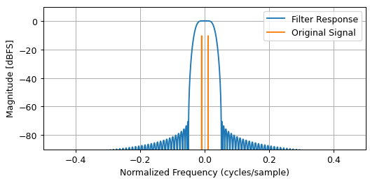
I created the following FIR filter using the least squares algorithm firls available in Python, Matlab and Octave. In Python done as (sig is from the scipy.signal package):

coeff = sig.firls(101, [0, .01, .05, .5], [1, 1, 0, 0], fs=1)

The frequency response for this filter is plotted below. The rejection and transition band is traded with the number of taps used.

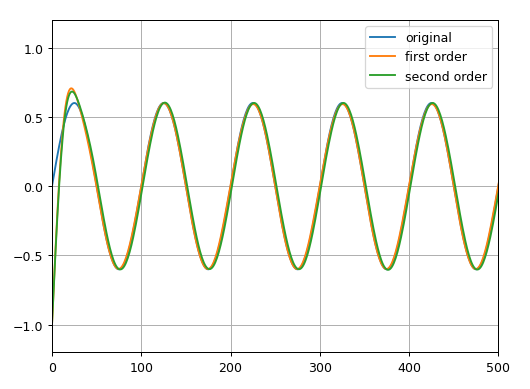
After filtering an extended (multi-cycle) version of the OP's waveform, using the following python command:

out1 = sig.filtfilt(coeff, 1, encoded)

I get the following result (where I also include a 2nd order version and dithering options explained further below).

It is important to note that a visual inspection such as above is not necessarily an adequate indication of how well we have recovered the waveform. Both a spectral evaluation on a dB scale, and an rms "error-vector-magnitude" (EVM) analysis will reveal much more about the quality of the reconstructed result. EVM is the measure of the rms error of the reconstructed waveform and its reference, importantly after matching delay and amplitude (a simple subtraction of input and output will not work since filtering used as well as the modulator itself can introduce fractional sample delays).

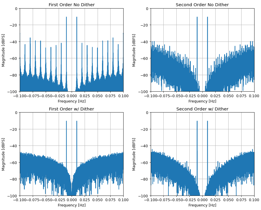
Important additional points are that the noise spectrum in a PDM waveform is "noise-shaped" in that the low frequency noise is suppressed at the expense of high frequency noise. Typically this would be a digital implementation as a delta sigma modulator and the noise would be the quantization noise from fixed precisions used. The improvement in noise significantly increases by the oversampling factor (how much we increase the sampling rate over Nyquist). The OP has implemented a simple first-order PDM, and with that the noise increases 6 dB/octave in the lower spectrum where a signal will occupy, resulting in a 9dB/octave improvement in SNR from oversampling. First order modulators are also prone to pattern noise resulting in very high spurious content in addition the desired waveform. This can be reduced through the addition of a "dither" to randomize the noise patterns as well as higher order modulations. I demonstrate both of these concepts with the additional 2nd order implementation below. A 2nd order implementation in comparison has a 12 dB/octave noise shaping and 15 dB/octave improvement in SNR from oversampling:

def pdm2(real_samples, dith_gain=0):
    # 2nd order pdm with dither
    res = []
    accum1 = 0
    accum2 = 0
    first_diff=0
    second_diff=0
    dither = np.random.randn(len(real_samples))
    for item, dith in zip(real_samples, dither):
        res.append(-1 if accum2 + dith * dith_gain <= 0 else 1)
        first_diff = item - res[-1]
        accum1 += first_diff
        second_diff = accum1 - 1.5 * res[-1] 
        accum2 += second_diff
return np.array(res)

With the following spectrum results below. Note that the input waveform should also be reduced from full scale which reduces the harmonic content (and ensures stability for the 2nd order implementation). The test signal for these was at 60% full scale and generated similar to the OP's code as:

N = 100
xs = np.linspace(0, 1000*2 * np.pi, N*1000)
ys = .6 * np.sin(xs)

I measured the EVM for the different cases above. Although the dither significantly reduces the harmonic content, the EVM will be better in the no-dither cases. With dither, we are adding noise (which reduces overall SNR and therefore EVM) at the benefit of decreasing the highest spur level, and therefore increases the spurious-free dynamic range.

EVM RESULTS (rms error):
1st order no dither (OP's original case): 2.05%
2nd order no dither: 0.59%
1st order with dither (dither gain=0.3): 2.8%
2nd order with dither (dither gain=0.3): 0.7%