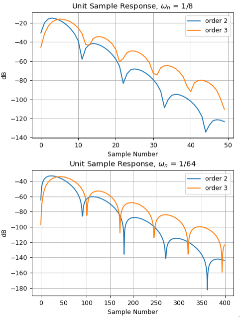
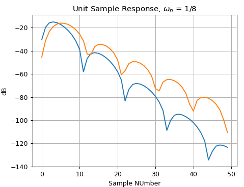
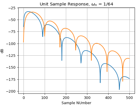
There is likely a closed form expression but what I do in the general case for any IIR filter including butterworth filters is use scipy.signal.unit_sampulse and plot the dB magnitude ofto evaluate the unit sample response for the filter on a dB scale (see Python example below). The “unit sample response” is the discrete-time equivalent of the “impulse response”. I then decide how good is “good enough” based on a distortion requirement (such as -80 or -100 dB) to then determine from that the number of samples to meet a given accuracy. The accuracy isof the result is the inverse of the distortion which we can get from: $20Log(1+10^{-d/20})$ where d is the distortion level in dB.
I commonly use this with any causal IIR filter to decide how many samples to truncate from the start of the output to avoid filter transients. The logic to doing this is very intuitive: from the impulse response we see how long the response from any particular slice from the input takes to decay to an insignificant value (based on our distortion criteria), which also is the time from when the first input and all previous inputs are stillwould be "valid" within our allowable error.
Below shows examples of this for the OP's butterworth 2nd and 3rd order filters and associated Python code:
import scipy.signal as sig
import matplotlib.pyplot as plt
plt.figure(figsize=(6,8))
plt.subplot(2,1,1)
imp = sig.unit_impulse(50)
for order in (2, 3):
    b, a = sig.butter(order, 1/8, 'lowpass')
    r = sig.lfilter(b,a,imp)
    plt.plot(20*np.log10(np.abs(r)), label = f"order {order}")
plt.title("Unit Sample Response, $\omega_n$ = 1/8")
plt.grid()
plt.xlabel("Sample Number")
plt.ylabel("dB")
plt.legend()

plt.subplot(2,1,2)
imp = sig.unit_impulse(400)
for order in (2, 3):
    b, a = sig.butter(order, 1/64, 'lowpass')
    r = sig.lfilter(b,a,imp)
    plt.plot(20*np.log10(np.abs(r)), label = f"order {order}")

plt.title("Unit Sample Response, $\omega_n$ = 1/64")
plt.grid()
plt.xlabel("Sample Number")
plt.ylabel("dB")
plt.legend()
plt.tight_layout()


