deleted 8 characters in body
Source Link

Algorithm

To encode a signal $x_m$ in a carrier with frequency $f_c$, we proceed as:

$$ y(t) = \cos(\phi(t)), \\ \phi(t) = 2\pi \cdot \left(f_c t + f_\Delta \int_0^t x_m(\tau)d\tau \right) $$

where $f_\Delta$ controls the maximum deviation of $y$'s instantaneous frequency from $f_c$ (effectively its bandwidth, but not in strict Fourier sense).

Discrete-time implementation is as follows:

  1. Integrate via cumulative sum
  2. Ensure $t$ is sampled properly per sampling frequency, i.e. $f_s = 1 / (t[1] - t[0])$. In Python this means linspace(t_min, t_max, N / (t_max - t_min), endpoint=False)
  3. Ensure $\phi(t)$ does not exceed $\pi$, adjusting $f_\Delta$ as necessary
  4. Ensure $f_c \leq f_s/2 - f_\Delta$, where $f_s$ is sampling frequency.

Applied example

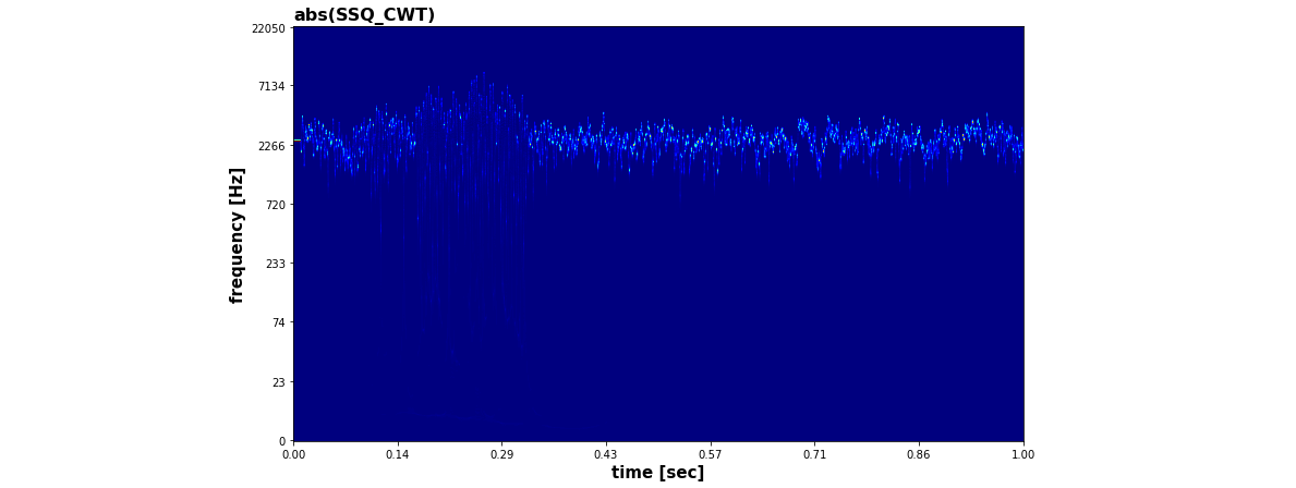
Doing all of the above for the first 1 second of OP's attached data yields below, which is validated with direct inspection, and using synchrosqueezed CWT with an extremely time-localized wavelet:

enter image description here

Zooming (note, CWT is logscale, so lower partit appears "stretched"):

enter image description here

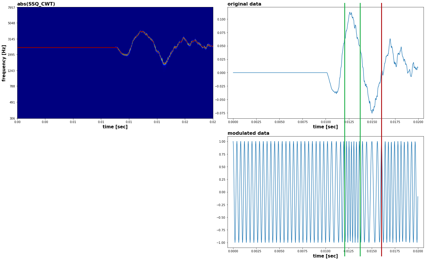
Zooming even more, and showing the result:

enter image description here

Code

Available at Github.

Algorithm

To encode a signal $x_m$ in a carrier with frequency $f_c$, we proceed as:

$$ y(t) = \cos(\phi(t)), \\ \phi(t) = 2\pi \cdot \left(f_c t + f_\Delta \int_0^t x_m(\tau)d\tau \right) $$

where $f_\Delta$ controls the maximum deviation of $y$'s instantaneous frequency from $f_c$ (effectively its bandwidth, but not in strict Fourier sense).

Discrete-time implementation is as follows:

  1. Integrate via cumulative sum
  2. Ensure $t$ is sampled properly per sampling frequency, i.e. $f_s = 1 / (t[1] - t[0])$. In Python this means linspace(t_min, t_max, N / (t_max - t_min), endpoint=False)
  3. Ensure $\phi(t)$ does not exceed $\pi$, adjusting $f_\Delta$ as necessary
  4. Ensure $f_c \leq f_s/2 - f_\Delta$, where $f_s$ is sampling frequency.

Applied example

Doing all of the above for the first 1 second of OP's attached data yields below, which is validated with direct inspection, and using synchrosqueezed CWT with an extremely time-localized wavelet:

enter image description here

Zooming (note, CWT is logscale, so lower part appears "stretched"):

enter image description here

Zooming even more, and showing the result:

enter image description here

Code

Available at Github.

Algorithm

To encode a signal $x_m$ in a carrier with frequency $f_c$, we proceed as:

$$ y(t) = \cos(\phi(t)), \\ \phi(t) = 2\pi \cdot \left(f_c t + f_\Delta \int_0^t x_m(\tau)d\tau \right) $$

where $f_\Delta$ controls the maximum deviation of $y$'s instantaneous frequency from $f_c$ (effectively its bandwidth, but not in strict Fourier sense).

Discrete-time implementation is as follows:

  1. Integrate via cumulative sum
  2. Ensure $t$ is sampled properly per sampling frequency, i.e. $f_s = 1 / (t[1] - t[0])$. In Python this means linspace(t_min, t_max, N / (t_max - t_min), endpoint=False)
  3. Ensure $\phi(t)$ does not exceed $\pi$, adjusting $f_\Delta$ as necessary
  4. Ensure $f_c \leq f_s/2 - f_\Delta$, where $f_s$ is sampling frequency.

Applied example

Doing all of the above for the first 1 second of OP's attached data yields below, which is validated with direct inspection, and using synchrosqueezed CWT with an extremely time-localized wavelet:

enter image description here

Zooming (note, CWT is logscale, so it appears "stretched"):

enter image description here

Zooming even more, and showing the result:

enter image description here

Code

Available at Github.

added 8 characters in body
Source Link

Algorithm

To encode a signal $x_m$ in a carrier with frequency $f_c$, we proceed as:

$$ y(t) = \cos(\phi(t)), \\ \phi(t) = 2\pi \cdot \left(f_c t + f_\Delta \int_0^t x_m(\tau)d\tau \right) $$

where $f_\Delta$ controls the maximum deviation of $y$'s instantaneous frequency from $f_c$ (effectively its bandwidth, but not in strict Fourier sense).

Discrete-time implementation is as follows:

  1. Integrate via cumulative sum
  2. Ensure $t$ is sampled properly per sampling frequency, i.e. $f_s = 1 / (t[1] - t[0])$. In Python this means linspace(t_min, t_max, N / (t_max - t_min), endpoint=False)
  3. Ensure $\phi(t)$ does not exceed $\pi$, adjusting $f_\Delta$ as necessary
  4. Ensure $f_c \leq f_s/2 - f_\Delta$, where $f_s$ is sampling frequency.

Applied example

Doing all of the above for the first 1 second of OP's attached data yields below, which is validated with direct inspection, and using synchrosqueezed CWT with an extremely time-localized wavelet:

enter image description here

Zooming (note, CWT is logscale, so lower part appears "stretched"):

enter image description here

Zooming even more, and showing the result:

enter image description here

Code

Available at GithubGithub.

Algorithm

To encode a signal $x_m$ in a carrier with frequency $f_c$, we proceed as:

$$ y(t) = \cos(\phi(t)), \\ \phi(t) = 2\pi \cdot \left(f_c t + f_\Delta \int_0^t x_m(\tau)d\tau \right) $$

where $f_\Delta$ controls the maximum deviation of $y$'s instantaneous frequency from $f_c$ (effectively its bandwidth, but not in strict Fourier sense).

Discrete-time implementation is as follows:

  1. Integrate via cumulative sum
  2. Ensure $t$ is sampled properly per sampling frequency, i.e. $f_s = 1 / (t[1] - t[0])$. In Python this means linspace(t_min, t_max, N / (t_max - t_min), endpoint=False)
  3. Ensure $\phi(t)$ does not exceed $\pi$, adjusting $f_\Delta$ as necessary
  4. Ensure $f_c \leq f_s/2 - f_\Delta$, where $f_s$ is sampling frequency.

Applied example

Doing all of the above for the first 1 second of OP's attached data yields below, which is validated with direct inspection, and using synchrosqueezed CWT with an extremely time-localized wavelet:

enter image description here

Zooming (note, CWT is logscale, so lower part appears "stretched"):

enter image description here

Zooming even more, and showing the result:

enter image description here

Code

Available at Github.

Source Link

Algorithm

To encode a signal $x_m$ in a carrier with frequency $f_c$, we proceed as:

$$ y(t) = \cos(\phi(t)), \\ \phi(t) = 2\pi \cdot \left(f_c t + f_\Delta \int_0^t x_m(\tau)d\tau \right) $$

where $f_\Delta$ controls the maximum deviation of $y$'s instantaneous frequency from $f_c$ (effectively its bandwidth, but not in strict Fourier sense).

Discrete-time implementation is as follows:

  1. Integrate via cumulative sum
  2. Ensure $t$ is sampled properly per sampling frequency, i.e. $f_s = 1 / (t[1] - t[0])$. In Python this means linspace(t_min, t_max, N / (t_max - t_min), endpoint=False)
  3. Ensure $\phi(t)$ does not exceed $\pi$, adjusting $f_\Delta$ as necessary
  4. Ensure $f_c \leq f_s/2 - f_\Delta$, where $f_s$ is sampling frequency.

Applied example

Doing all of the above for the first 1 second of OP's attached data yields below, which is validated with direct inspection, and using synchrosqueezed CWT with an extremely time-localized wavelet:

enter image description here

Zooming (note, CWT is logscale, so lower part appears "stretched"):

enter image description here

Zooming even more, and showing the result:

enter image description here

Code

Available at Github.