added 85 characters in body
Source Link

Since I don't have sufficient reputation to comment i will quote and add to Dsp_user's answer.

Summary: The error variance will depend onhow well you can estimate the frequency of your signal. This in turn will be limited by the amplitude of the DFT peak vs noise level. Spectral leakage will likely also skew your estimates.

the latter can't be assigned a physical meaning (please someone correct me if I'm wrong on this point).

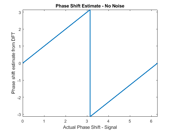
this is incorrect, calculated phase from the DFT is linearly correlated with phase shift of a sinusoid. When generating a cosinus curve and shift it between 0:2*pi i get errors in the range of (10^-15) between signal phase shift and phase estimate. Phase estimates from DFT can thus be said to compare a signals shift to a non-shifted signal. Simulated curve is shown bellow:

enter image description here

In my opinion, phase estimation error should only be dependent on how well the "sinusoidal-fit" from the DFT fits the actual signal. One of those limitations (frequency resolution/spectral leakage) was explained by Dsp_user. If your signal is between frequency bins you will estimate the wrong signal amplitude (correlated with how close the frequency is to the middle between two bins). Since phase estimation by DFT is linerly dependent on signal frequency i would guess that you will introduce a higher/lower derivative when trying to estimate real time shifts between signals but I admit here that I am not 100%.

Added: In case of spectral leakage, if you have other sinusoids close to your peak of interest, their leakage could pour onto that and introduce errors.

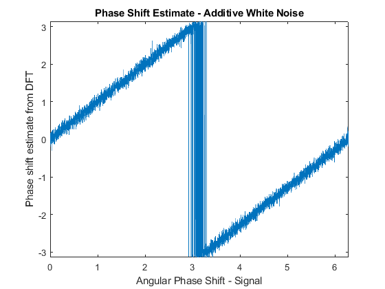
Your noise floor (if it is white) will in real cases likely be your largest source of error. It will cause additive errors to your phase estimates whose size will depend on DFT-Peak Amplitude vs noise floor amplitude (noise power spread out over the signal length). Bellow you can find a figure of this as well as the code to generate both in my answer

enter image description here

t=0:1000^-1:.999;
phi=0:1000^-1:2*pi-1000^-1;
signal = cos(2*pi*10*t+phi');

FFTSig= fft(signal,[],2);
figure; plot(phi,squeeze(atan2(imag(FFTSig(:,11)),real(FFTSig(:,11)))),'linewidth',2)
xlim([0 2*pi])
ylim([-pi pi])
xlabel('Signal Phase Shift')
ylabel('Phase shift estimate from DFT')
title('Phase Shift Estimate - No Noise')

signal2 = cos(2*pi*10*t+phi');
for iter=1:6283
   signal2(iter,:)= squeeze(signal2(iter,:))+2*randn(length(signal(1,:)),1)';
end

FFTSig2= fft(signal2,[],2);
figure; plot(phi,squeeze(atan2(imag(FFTSig2(:,11)),real(FFTSig2(:,11)))))
xlim([0 2*pi])
ylim([-pi pi])
xlabel('Signal Phase Shift')
ylabel('Phase shift estimate from DFT')
title('Phase Shift Estimate - Additive White Noise')

Since I don't have sufficient reputation to comment i will quote and add to Dsp_user's answer.

Summary: The error variance will depend on the amplitude of the DFT peak vs noise level. Spectral leakage will likely also skew your estimates.

the latter can't be assigned a physical meaning (please someone correct me if I'm wrong on this point).

this is incorrect, calculated phase from the DFT is linearly correlated with phase shift of a sinusoid. When generating a cosinus curve and shift it between 0:2*pi i get errors in the range of (10^-15) between signal phase shift and phase estimate. Phase estimates from DFT can thus be said to compare a signals shift to a non-shifted signal. Simulated curve is shown bellow:

enter image description here

In my opinion, phase estimation error should only be dependent on how well the "sinusoidal-fit" from the DFT fits the actual signal. One of those limitations (frequency resolution/spectral leakage) was explained by Dsp_user. If your signal is between frequency bins you will estimate the wrong signal amplitude (correlated with how close the frequency is to the middle between two bins). Since phase estimation by DFT is linerly dependent on signal frequency i would guess that you will introduce a higher/lower derivative when trying to estimate real time shifts between signals but I admit here that I am not 100%.

Added: In case of spectral leakage, if you have other sinusoids close to your peak of interest, their leakage could pour onto that and introduce errors.

Your noise floor (if it is white) will in real cases likely be your largest source of error. It will cause additive errors to your phase estimates whose size will depend on DFT-Peak Amplitude vs noise floor amplitude (noise power spread out over the signal length). Bellow you can find a figure of this as well as the code to generate both in my answer

enter image description here

t=0:1000^-1:.999;
phi=0:1000^-1:2*pi-1000^-1;
signal = cos(2*pi*10*t+phi');

FFTSig= fft(signal,[],2);
figure; plot(phi,squeeze(atan2(imag(FFTSig(:,11)),real(FFTSig(:,11)))),'linewidth',2)
xlim([0 2*pi])
ylim([-pi pi])
xlabel('Signal Phase Shift')
ylabel('Phase shift estimate from DFT')
title('Phase Shift Estimate - No Noise')

signal2 = cos(2*pi*10*t+phi');
for iter=1:6283
   signal2(iter,:)= squeeze(signal2(iter,:))+2*randn(length(signal(1,:)),1)';
end

FFTSig2= fft(signal2,[],2);
figure; plot(phi,squeeze(atan2(imag(FFTSig2(:,11)),real(FFTSig2(:,11)))))
xlim([0 2*pi])
ylim([-pi pi])
xlabel('Signal Phase Shift')
ylabel('Phase shift estimate from DFT')
title('Phase Shift Estimate - Additive White Noise')
Since I don't have sufficient reputation to comment i will quote and add to Dsp_user's answer.

Summary: The error variance will depend how well you can estimate the frequency of your signal. This in turn will be limited by the amplitude of the DFT peak vs noise level. Spectral leakage will likely also skew your estimates.

the latter can't be assigned a physical meaning (please someone correct me if I'm wrong on this point).

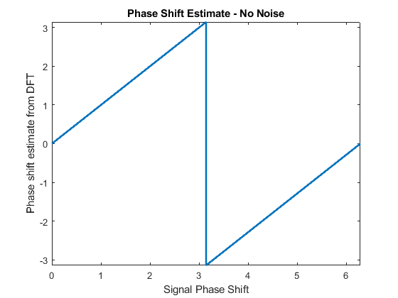
this is incorrect, calculated phase from the DFT is linearly correlated with phase shift of a sinusoid. When generating a cosinus curve and shift it between 0:2*pi i get errors in the range of (10^-15) between signal phase shift and phase estimate. Phase estimates from DFT can thus be said to compare a signals shift to a non-shifted signal. Simulated curve is shown bellow:

enter image description here

In my opinion, phase estimation error should only be dependent on how well the "sinusoidal-fit" from the DFT fits the actual signal. One of those limitations (frequency resolution/spectral leakage) was explained by Dsp_user. If your signal is between frequency bins you will estimate the wrong signal amplitude (correlated with how close the frequency is to the middle between two bins). Since phase estimation by DFT is linerly dependent on signal frequency i would guess that you will introduce a higher/lower derivative when trying to estimate real time shifts between signals but I admit here that I am not 100%.

Added: In case of spectral leakage, if you have other sinusoids close to your peak of interest, their leakage could pour onto that and introduce errors.

Your noise floor (if it is white) will in real cases likely be your largest source of error. It will cause additive errors to your phase estimates whose size will depend on DFT-Peak Amplitude vs noise floor amplitude (noise power spread out over the signal length). Bellow you can find a figure of this as well as the code to generate both in my answer

enter image description here

t=0:1000^-1:.999;
phi=0:1000^-1:2*pi-1000^-1;
signal = cos(2*pi*10*t+phi');

FFTSig= fft(signal,[],2);
figure; plot(phi,squeeze(atan2(imag(FFTSig(:,11)),real(FFTSig(:,11)))),'linewidth',2)
xlim([0 2*pi])
ylim([-pi pi])
xlabel('Signal Phase Shift')
ylabel('Phase shift estimate from DFT')
title('Phase Shift Estimate - No Noise')

signal2 = cos(2*pi*10*t+phi');
for iter=1:6283
   signal2(iter,:)= squeeze(signal2(iter,:))+2*randn(length(signal(1,:)),1)';
end

FFTSig2= fft(signal2,[],2);
figure; plot(phi,squeeze(atan2(imag(FFTSig2(:,11)),real(FFTSig2(:,11)))))
xlim([0 2*pi])
ylim([-pi pi])
xlabel('Signal Phase Shift')
ylabel('Phase shift estimate from DFT')
title('Phase Shift Estimate - Additive White Noise')
added 3 characters in body
Source Link

Since I don't have sufficient reputation to comment i will quote and add to Dsp_user's answer.

Summary: The error variance will depend on the amplitude of the DFT peak vs noise level. Spectral leakage will likely also skew your estimates.

the latter can't be assigned a physical meaning (please someone correct me if I'm wrong on this point).

this is incorrect, calculated phase from the DFT is linearly correlated with phase shift of a sinusoid. When generating a cosinus curve and shift it between 0:2*pi i get errors in the range of (10^-15) between signal phase shift and phase estimate. Phase estimates from DFT can thus be said to compare a signals shift to a non-shifted signal. Simulated curve is shown bellow:

enter image description here

In my opinion, phase estimation error should only be dependent on how well the "sinusoidal-fit" from the DFT fits the actual signal. One of those limitations (frequency resolution/spectral leakage) was explained by Dsp_user. If your signal is between frequency bins you will estimate the wrong signal amplitude (correlated with how close the frequency is to the middle between two bins). Since phase estimation by DFT is linerly dependent on signal frequency i would guess that you will introduce a higher/lower derivative when trying to estimate real time shifts between signals but I admit here that I am not 100%.

Added: In case of spectral leakage, if you have other sinusoids close byto your peak of interest, their leakage could pour onto your frequency of interestthat and introduce errors.

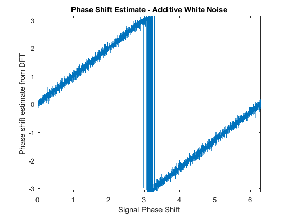
Your noise floor (if it is white) will in real cases likely be your largest source of error. It will cause additive errors to your phase estimates whose size will depend on DFT-Peak Amplitude vs noise floor amplitude (noise power spread out over the signal length). Bellow you can find a simulationfigure of this as well as the code to generate both imagesin my answer

enter image description here

t=0:1000^-1:.999;
phi=0:1000^-1:2*pi-1000^-1;
signal = cos(2*pi*10*t+phi');

FFTSig= fft(signal,[],2);
figure; plot(phi,squeeze(atan2(imag(FFTSig(:,11)),real(FFTSig(:,11)))),'linewidth',2)
xlim([0 2*pi])
ylim([-pi pi])
xlabel('Signal Phase Shift')
ylabel('Phase shift estimate from DFT')
title('Phase Shift Estimate - No Noise')

signal2 = cos(2*pi*10*t+phi');
for iter=1:6283
   signal2(iter,:)= squeeze(signal2(iter,:))+2*randn(length(signal(1,:)),1)';
end

FFTSig2= fft(signal2,[],2);
figure; plot(phi,squeeze(atan2(imag(FFTSig2(:,11)),real(FFTSig2(:,11)))))
xlim([0 2*pi])
ylim([-pi pi])
xlabel('Signal Phase Shift')
ylabel('Phase shift estimate from DFT')
title('Phase Shift Estimate - Additive White Noise')
Since I don't have sufficient reputation to comment i will quote and add to Dsp_user's answer.

Summary: The error variance will depend on the amplitude of the DFT peak vs noise level. Spectral leakage will likely also skew your estimates.

the latter can't be assigned a physical meaning (please someone correct me if I'm wrong on this point).

this is incorrect, calculated phase from the DFT is linearly correlated with phase shift of a sinusoid. When generating a cosinus curve and shift it between 0:2*pi i get errors in the range of (10^-15) between signal phase shift and phase estimate. Phase estimates from DFT can thus be said to compare a signals shift to a non-shifted signal. Simulated curve is shown bellow:

enter image description here

In my opinion, phase estimation error should only be dependent on how well the "sinusoidal-fit" from the DFT fits the actual signal. One of those limitations (frequency resolution/spectral leakage) was explained by Dsp_user. If your signal is between frequency bins you will estimate the wrong signal amplitude (correlated with how close the frequency is to the middle between two bins). Since phase estimation by DFT is linerly dependent on signal frequency i would guess that you will introduce a higher/lower derivative when trying to estimate real time shifts between signals but I admit here that I am not 100%.

Added: In case of spectral leakage, if you have other sinusoids close by, their leakage could pour onto your frequency of interest and introduce errors.

Your noise floor (if it is white) will in real cases likely be your largest source of error. It will cause additive errors to your phase estimates whose size will depend on DFT-Peak Amplitude vs noise floor amplitude (noise power spread out over the signal length). Bellow you can find a simulation of this as well as the code to generate both images

enter image description here

t=0:1000^-1:.999;
phi=0:1000^-1:2*pi-1000^-1;
signal = cos(2*pi*10*t+phi');

FFTSig= fft(signal,[],2);
figure; plot(phi,squeeze(atan2(imag(FFTSig(:,11)),real(FFTSig(:,11)))),'linewidth',2)
xlim([0 2*pi])
ylim([-pi pi])
xlabel('Signal Phase Shift')
ylabel('Phase shift estimate from DFT')
title('Phase Shift Estimate - No Noise')

signal2 = cos(2*pi*10*t+phi');
for iter=1:6283
   signal2(iter,:)= squeeze(signal2(iter,:))+2*randn(length(signal(1,:)),1)';
end

FFTSig2= fft(signal2,[],2);
figure; plot(phi,squeeze(atan2(imag(FFTSig2(:,11)),real(FFTSig2(:,11)))))
xlim([0 2*pi])
ylim([-pi pi])
xlabel('Signal Phase Shift')
ylabel('Phase shift estimate from DFT')
title('Phase Shift Estimate - Additive White Noise')

Since I don't have sufficient reputation to comment i will quote and add to Dsp_user's answer.

Summary: The error variance will depend on the amplitude of the DFT peak vs noise level. Spectral leakage will likely also skew your estimates.

the latter can't be assigned a physical meaning (please someone correct me if I'm wrong on this point).

this is incorrect, calculated phase from the DFT is linearly correlated with phase shift of a sinusoid. When generating a cosinus curve and shift it between 0:2*pi i get errors in the range of (10^-15) between signal phase shift and phase estimate. Phase estimates from DFT can thus be said to compare a signals shift to a non-shifted signal. Simulated curve is shown bellow:

enter image description here

In my opinion, phase estimation error should only be dependent on how well the "sinusoidal-fit" from the DFT fits the actual signal. One of those limitations (frequency resolution/spectral leakage) was explained by Dsp_user. If your signal is between frequency bins you will estimate the wrong signal amplitude (correlated with how close the frequency is to the middle between two bins). Since phase estimation by DFT is linerly dependent on signal frequency i would guess that you will introduce a higher/lower derivative when trying to estimate real time shifts between signals but I admit here that I am not 100%.

Added: In case of spectral leakage, if you have other sinusoids close to your peak of interest, their leakage could pour onto that and introduce errors.

Your noise floor (if it is white) will in real cases likely be your largest source of error. It will cause additive errors to your phase estimates whose size will depend on DFT-Peak Amplitude vs noise floor amplitude (noise power spread out over the signal length). Bellow you can find a figure of this as well as the code to generate both in my answer

enter image description here

t=0:1000^-1:.999;
phi=0:1000^-1:2*pi-1000^-1;
signal = cos(2*pi*10*t+phi');

FFTSig= fft(signal,[],2);
figure; plot(phi,squeeze(atan2(imag(FFTSig(:,11)),real(FFTSig(:,11)))),'linewidth',2)
xlim([0 2*pi])
ylim([-pi pi])
xlabel('Signal Phase Shift')
ylabel('Phase shift estimate from DFT')
title('Phase Shift Estimate - No Noise')

signal2 = cos(2*pi*10*t+phi');
for iter=1:6283
   signal2(iter,:)= squeeze(signal2(iter,:))+2*randn(length(signal(1,:)),1)';
end

FFTSig2= fft(signal2,[],2);
figure; plot(phi,squeeze(atan2(imag(FFTSig2(:,11)),real(FFTSig2(:,11)))))
xlim([0 2*pi])
ylim([-pi pi])
xlabel('Signal Phase Shift')
ylabel('Phase shift estimate from DFT')
title('Phase Shift Estimate - Additive White Noise')
added 3 characters in body
Source Link

Since I don't have sufficient reputation to comment i will quote and add to Dsp_usersDsp_user's answer.

Summary: The error variance will depend on the amplitude of the DFT peak vs noise level. Spectral leakage will likely also skew your estimates.

the latter can't be assigned a physical meaning (please someone correct me if I'm wrong on this point).

this is incorrect, calculated phase from the DFT is linearly correlated with phase shift of a sinusoid. When generating a cosinus curve and shift it between 0:2*pi i get errors in the range of (10^-15) between signal phase shift and phase estimate. Phase estimates from DFT can thus be said to compare a signals shift to a non-shifted signal. Simulated curve is shown bellow:

enter image description hereenter image description here

In my opinion, (relevant) phase estimation error should only be dependent on how well the "sinusoidal-fit" from the DFT fits the actual signal. One of those limitations (frequency resolution/spectral leakage) was explained by Dsp_user. If your signal is between frequency bins you will estimate the wrong signal amplitude (correlated with how close the frequency is to the middle between two bins). Since phase estimation by DFT is linerly dependent on signal frequency i would guess that you will introduce a higher/lower derivative when trying to estimate real time shifts between signals but I admit here that I am not 100%.

Added: In case of spectral leakage, if you have other sinusoids close by, their leakage could pour onto your frequency of interest and introduce errors.

Your noise floor (if it is white) will in real cases likely be your largest source of error. It will cause additive errors to your phase estimates whose size will depend on DFT-Peak Amplitude vs noise floor amplitude (noise power spread out over the signal length). Bellow you can find a simulation of this as well as the code to generate both images

enter image description hereenter image description here

t=0:1000^-1:.999;
phi=0:1000^-1:2*pi-1000^-1;
signal = cos(2*pi*10*t+phi');

FFTSig= fft(signal,[],2);
figure; plot(phi,squeeze(atan2(imag(FFTSig(:,11)),real(FFTSig(:,11)))),'linewidth',2)
xlim([0 2*pi])
ylim([-pi pi])
xlabel('Signal Phase Shift')
ylabel('Phase shift estimate from DFT')
title('Phase Shift Estimate - No Noise')

signal2 = cos(2*pi*10*t+phi');
for iter=1:6283
   signal2(iter,:)= squeeze(signal2(iter,:))+2*randn(length(signal(1,:)),1)';
end

FFTSig2= fft(signal2,[],2);
figure; plot(phi,squeeze(atan2(imag(FFTSig2(:,11)),real(FFTSig2(:,11)))))
xlim([0 2*pi])
ylim([-pi pi])
xlabel('Signal Phase Shift')
ylabel('Phase shift estimate from DFT')
title('Phase Shift Estimate - Additive White Noise')

Since I don't have sufficient reputation to comment i will quote and add to Dsp_users answer.

the latter can't be assigned a physical meaning (please someone correct me if I'm wrong on this point).

this is incorrect, calculated phase from the DFT is linearly correlated with phase shift of a sinusoid. When generating a cosinus curve and shift it between 0:2*pi i get errors in the range of (10^-15) between signal phase shift and phase estimate. Phase estimates from DFT can thus be said to compare a signals shift to a non-shifted signal. Simulated curve is shown bellow:

enter image description here

In my opinion, (relevant) phase estimation error should only be dependent on how well the "sinusoidal-fit" from the DFT fits the actual signal. One of those limitations (frequency resolution/spectral leakage) was explained by Dsp_user. If your signal is between frequency bins you will estimate the wrong signal amplitude (correlated with how close the frequency is to the middle between two bins). Since phase estimation by DFT is linerly dependent on signal frequency i would guess that you will introduce a higher/lower derivative when trying to estimate real time shifts between signals but I admit here that I am not 100%.

Added: In case of spectral leakage, if you have other sinusoids close by, their leakage could pour onto your frequency of interest and introduce errors.

Your noise floor (if it is white) will in real cases likely be your largest source of error. It will cause additive errors to your phase estimates whose size will depend on DFT-Peak Amplitude vs noise floor amplitude (noise power spread out over the signal length). Bellow you can find a simulation of this as well as the code to generate both images

enter image description here

t=0:1000^-1:.999;
phi=0:1000^-1:2*pi-1000^-1;
signal = cos(2*pi*10*t+phi');

FFTSig= fft(signal,[],2);
figure; plot(phi,squeeze(atan2(imag(FFTSig(:,11)),real(FFTSig(:,11)))),'linewidth',2)
xlim([0 2*pi])
ylim([-pi pi])
xlabel('Signal Phase Shift')
ylabel('Phase shift estimate from DFT')
title('Phase Shift Estimate - No Noise')

signal2 = cos(2*pi*10*t+phi');
for iter=1:6283
   signal2(iter,:)= squeeze(signal2(iter,:))+2*randn(length(signal(1,:)),1)';
end

FFTSig2= fft(signal2,[],2);
figure; plot(phi,squeeze(atan2(imag(FFTSig2(:,11)),real(FFTSig2(:,11)))))
xlim([0 2*pi])
ylim([-pi pi])
xlabel('Signal Phase Shift')
ylabel('Phase shift estimate from DFT')
title('Phase Shift Estimate - Additive White Noise')

Since I don't have sufficient reputation to comment i will quote and add to Dsp_user's answer.

Summary: The error variance will depend on the amplitude of the DFT peak vs noise level. Spectral leakage will likely also skew your estimates.

the latter can't be assigned a physical meaning (please someone correct me if I'm wrong on this point).

this is incorrect, calculated phase from the DFT is linearly correlated with phase shift of a sinusoid. When generating a cosinus curve and shift it between 0:2*pi i get errors in the range of (10^-15) between signal phase shift and phase estimate. Phase estimates from DFT can thus be said to compare a signals shift to a non-shifted signal. Simulated curve is shown bellow:

enter image description here

In my opinion, phase estimation error should only be dependent on how well the "sinusoidal-fit" from the DFT fits the actual signal. One of those limitations (frequency resolution/spectral leakage) was explained by Dsp_user. If your signal is between frequency bins you will estimate the wrong signal amplitude (correlated with how close the frequency is to the middle between two bins). Since phase estimation by DFT is linerly dependent on signal frequency i would guess that you will introduce a higher/lower derivative when trying to estimate real time shifts between signals but I admit here that I am not 100%.

Added: In case of spectral leakage, if you have other sinusoids close by, their leakage could pour onto your frequency of interest and introduce errors.

Your noise floor (if it is white) will in real cases likely be your largest source of error. It will cause additive errors to your phase estimates whose size will depend on DFT-Peak Amplitude vs noise floor amplitude (noise power spread out over the signal length). Bellow you can find a simulation of this as well as the code to generate both images

enter image description here

t=0:1000^-1:.999;
phi=0:1000^-1:2*pi-1000^-1;
signal = cos(2*pi*10*t+phi');

FFTSig= fft(signal,[],2);
figure; plot(phi,squeeze(atan2(imag(FFTSig(:,11)),real(FFTSig(:,11)))),'linewidth',2)
xlim([0 2*pi])
ylim([-pi pi])
xlabel('Signal Phase Shift')
ylabel('Phase shift estimate from DFT')
title('Phase Shift Estimate - No Noise')

signal2 = cos(2*pi*10*t+phi');
for iter=1:6283
   signal2(iter,:)= squeeze(signal2(iter,:))+2*randn(length(signal(1,:)),1)';
end

FFTSig2= fft(signal2,[],2);
figure; plot(phi,squeeze(atan2(imag(FFTSig2(:,11)),real(FFTSig2(:,11)))))
xlim([0 2*pi])
ylim([-pi pi])
xlabel('Signal Phase Shift')
ylabel('Phase shift estimate from DFT')
title('Phase Shift Estimate - Additive White Noise')
Source Link
Loading