Thank you so much everyone!

I am really not confident in my mathematics skills and so I was focusing on the Fourrier transform, but as you all guessed, the problem was my way too small sampling frequency (I was using 25kHz). With 60kHz it works like a charm. Still feels like an idiot though ;-)

Thank you !

PS : To sum up if anyone was facing the same kind of problem

The theoric part was wright. We have : $$\delta(f) +\frac 18 \bigg[\delta(f-3f_0)+\delta(f-3f_0)\bigg] +\frac 38 \bigg[\delta(f-f_0)+\delta(f-f_0)\bigg]$$

The problem was with my simulation: I forgot to check if my sampling frequency was meeting the Nyquist-Shannon criteria ($Fs > 2F_{max}$).

So, with this code :

Fs = 7e4;            % Sampling frequency
T = 1/Fs;             % Sampling period
L = 100000;             % Length of signal
t = (0:L-1)*T;        % Time vector
fm = 10e3;

X = 1+(cos(2*pi*fm*t)).^3;
%X = 1 + 0.25*cos(3*2*pi*10000*t)+(3/4)*cos(2*pi*10000*t);
Y = abs(fft(X));

f = 0:Fs/L:Fs/2;
plot(f,Y(1:L/2+1))
xlabel('f (Hz)')
ylabel('|P1(f)|')

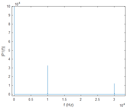
We get the expected result:

Thank you so much everyone!

I am really not confident in my mathematics skills and so I was focusing on the Fourier transform, but as you all guessed, the problem was my sampling frequency way too small (I was using 25kHz). With 60kHz it works like a charm. Still feels like an idiot though ;-)

Thank you !

PS : To sum up if anyone was facing the same kind of problem

The theoric part was wright. We have : $$\delta(f) +\frac 18 \bigg[\delta(f-3f_0)+\delta(f-3f_0)\bigg] +\frac 38 \bigg[\delta(f-f_0)+\delta(f-f_0)\bigg]$$

The problem was with my simulation: I forgot to check if my sampling frequency was meeting the Nyquist-Shannon criteria ($Fs > 2F_{max}$).

So, with this code :

Fs = 7e4;            % Sampling frequency
T = 1/Fs;             % Sampling period
L = 100000;             % Length of signal
t = (0:L-1)*T;        % Time vector
fm = 10e3;

X = 1+(cos(2*pi*fm*t)).^3;
%X = 1 + 0.25*cos(3*2*pi*10000*t)+(3/4)*cos(2*pi*10000*t);
Y = abs(fft(X));

f = 0:Fs/L:Fs/2;
plot(f,Y(1:L/2+1))
xlabel('f (Hz)')
ylabel('|P1(f)|')

We get the expected result:

Thank you so much everyone  !

I am really not confident in my mathematics skills and so I was focusing on the Fourrier transform, but as you all guessed, the problem was my way too small sampling frequency (I was using 25kHz). With 60kHz it works like a charm. Still feels like an idiot though ;-)

Thank you !

PS : To sum up if anyone was facing the same kind of problem

The theoric part was wright. We have : $$\delta(f) +\frac 18 \bigg[\delta(f-3f_0)+\delta(f-3f_0)\bigg] +\frac 38 \bigg[\delta(f-f_0)+\delta(f-f_0)\bigg]$$

The problem was with my simulation: I forgot to check if my sampling frequency was meeting the Nyquist-Shannon criteria ($Fs > 2F_{max}$).

So, with this code :

Fs = 7e4;            % Sampling frequency
T = 1/Fs;             % Sampling period
L = 100000;             % Length of signal
t = (0:L-1)*T;        % Time vector
fm = 10e3;

X = 1+(cos(2*pi*fm*t)).^3;
%X = 1 + 0.25*cos(3*2*pi*10000*t)+(3/4)*cos(2*pi*10000*t);
Y = abs(fft(X));

f = 0:Fs/L:Fs/2;
plot(f,Y(1:L/2+1))
xlabel('f (Hz)')
ylabel('|P1(f)|')

We get the expected result:

Thank you so much everyone!

I am really not confident in my mathematics skills and so I was focusing on the Fourrier transform, but as you all guessed, the problem was my way too small sampling frequency (I was using 25kHz). With 60kHz it works like a charm. Still feels like an idiot though ;-)

Thank you !

PS : To sum up if anyone was facing the same kind of problem

The theoric part was wright. We have : $$\delta(f) +\frac 18 \bigg[\delta(f-3f_0)+\delta(f-3f_0)\bigg] +\frac 38 \bigg[\delta(f-f_0)+\delta(f-f_0)\bigg]$$

The problem was with my simulation: I forgot to check if my sampling frequency was meeting the Nyquist-Shannon criteria ($Fs > 2F_{max}$).

So, with this code :

Fs = 7e4;            % Sampling frequency
T = 1/Fs;             % Sampling period
L = 100000;             % Length of signal
t = (0:L-1)*T;        % Time vector
fm = 10e3;

X = 1+(cos(2*pi*fm*t)).^3;
%X = 1 + 0.25*cos(3*2*pi*10000*t)+(3/4)*cos(2*pi*10000*t);
Y = abs(fft(X));

f = 0:Fs/L:Fs/2;
plot(f,Y(1:L/2+1))
xlabel('f (Hz)')
ylabel('|P1(f)|')

We get the expected result: