deleted 1 character in body
Source Link
Royi
  • 20.5k
  • 4
  • 199
  • 240

I will divide my answer into 3 sections.

The Distribution of the Derivative of Images

Take a real world image, any image.
Apply the derivative operator on it (Namely apply the kernel $ \left[ 1, -1 \right] $ on it.
Display the histogram of the filtered image.

I took this image:

enter image description here

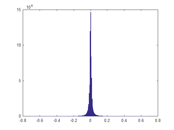
The histogram I got is this:

enter image description here

This distribution is very similar to Laplace Distribution.
Clearly, this distribution is "Sparse" namely most of the values are 0 (Or close) and very few are different.
In real world we assume most of the values which are small yet not zero are actually due to the noise.

Total Variation Optimization Problem

Look at the Optimization Function:

$$ \hat{x} = \arg \min_{x} {\| Hx -y \|}^{2} + \lambda {\| G x \|}_{1} $$

Where $ H $ is the Blur Operator and $ G $ is the Derivative Operator.

Now, you can look at it in the Sparse sense or you can look at it as the MAP solution given a Laplace prior for the Gradient.

As written above, it fits very well to real world images.

Sparse Optimization

Look at the Optimization Function:

$$ \hat{x} = \arg \min_{x} {\| Hx -y \|}^{2} + \lambda {\| G x \|}_{0} $$

Where $ H $ is the Blur Operator and $ G $ is the Derivative Operator.

This optimization problem clearly promote Sparse solution (With respect to the Derivative).
Yet, this is a very hard problem to solve.
Hence it was shown that under some circumstances the solution of the problem with $ {\ell}_{1} $ coincide with this solution.

Moreover, by looking at the Unit Sphere o fof different norms (And the Pseudo Norm $ {\ell}_{o} $, or more correctly Cardinality Function) you can see why the lower the norm the Sparse Solution it promotes.

All in all you have many point of view on the same problem.

I will divide my answer into 3 sections.

The Distribution of the Derivative of Images

Take a real world image, any image.
Apply the derivative operator on it (Namely apply the kernel $ \left[ 1, -1 \right] $ on it.
Display the histogram of the filtered image.

I took this image:

enter image description here

The histogram I got is this:

enter image description here

This distribution is very similar to Laplace Distribution.
Clearly, this distribution is "Sparse" namely most of the values are 0 (Or close) and very few are different.
In real world we assume most of the values which are small yet not zero are actually due to the noise.

Total Variation Optimization Problem

Look at the Optimization Function:

$$ \hat{x} = \arg \min_{x} {\| Hx -y \|}^{2} + \lambda {\| G x \|}_{1} $$

Where $ H $ is the Blur Operator and $ G $ is the Derivative Operator.

Now, you can look at it in the Sparse sense or you can look at it as the MAP solution given a Laplace prior for the Gradient.

As written above, it fits very well to real world images.

Sparse Optimization

Look at the Optimization Function:

$$ \hat{x} = \arg \min_{x} {\| Hx -y \|}^{2} + \lambda {\| G x \|}_{0} $$

Where $ H $ is the Blur Operator and $ G $ is the Derivative Operator.

This optimization problem clearly promote Sparse solution (With respect to the Derivative).
Yet, this is a very hard problem to solve.
Hence it was shown that under some circumstances the solution of the problem with $ {\ell}_{1} $ coincide with this solution.

Moreover, by looking at the Unit Sphere o f different norms (And the Pseudo Norm $ {\ell}_{o} $, or more correctly Cardinality Function) you can see why the lower the norm the Sparse Solution it promotes.

All in all you have many point of view on the same problem.

I will divide my answer into 3 sections.

The Distribution of the Derivative of Images

Take a real world image, any image.
Apply the derivative operator on it (Namely apply the kernel $ \left[ 1, -1 \right] $ on it.
Display the histogram of the filtered image.

I took this image:

enter image description here

The histogram I got is this:

enter image description here

This distribution is very similar to Laplace Distribution.
Clearly, this distribution is "Sparse" namely most of the values are 0 (Or close) and very few are different.
In real world we assume most of the values which are small yet not zero are actually due to the noise.

Total Variation Optimization Problem

Look at the Optimization Function:

$$ \hat{x} = \arg \min_{x} {\| Hx -y \|}^{2} + \lambda {\| G x \|}_{1} $$

Where $ H $ is the Blur Operator and $ G $ is the Derivative Operator.

Now, you can look at it in the Sparse sense or you can look at it as the MAP solution given a Laplace prior for the Gradient.

As written above, it fits very well to real world images.

Sparse Optimization

Look at the Optimization Function:

$$ \hat{x} = \arg \min_{x} {\| Hx -y \|}^{2} + \lambda {\| G x \|}_{0} $$

Where $ H $ is the Blur Operator and $ G $ is the Derivative Operator.

This optimization problem clearly promote Sparse solution (With respect to the Derivative).
Yet, this is a very hard problem to solve.
Hence it was shown that under some circumstances the solution of the problem with $ {\ell}_{1} $ coincide with this solution.

Moreover, by looking at the Unit Sphere of different norms (And the Pseudo Norm $ {\ell}_{o} $, or more correctly Cardinality Function) you can see why the lower the norm the Sparse Solution it promotes.

All in all you have many point of view on the same problem.
added 40 characters in body
Source Link
Royi
  • 20.5k
  • 4
  • 199
  • 240

I will divide my answer into 3 sections.

The Distribution of the Derivative of Images

Take a real world image, any image.
Apply the derivative operator on it (Namely apply the kernel $ \left[ 1, -1 \right] $ on it.
Display the histogram of the filtered image.

I took this image:

enter image description here

The histogram I got is this:

enter image description here

This distribution is very similar to Laplace Distribution.
Clearly, this distribution is "Sparse" namely most of the values are 0 (Or close) and very few are different.
In real world we assume most of the values which are small yet not zero are actually due to the noise.

Total Variation Optimization Problem

Look at the Optimization Function:

$$ \hat{x} = \arg \min_{x} {\| Hx -y \|}^{2} + \lambda {\| G x \|}_{1} $$

Where $ H $ is the Blur Operator and $ G $ is the Derivative Operator.

Now, you can look at it in the Sparse sense or you can look at it as the MAP solution given a Laplace prior for the Gradient.

As written above, it fits very well to real world images.

Sparse Optimization

Look at the Optimization Function:

$$ \hat{x} = \arg \min_{x} {\| Hx -y \|}^{2} + \lambda {\| G x \|}_{0} $$

Where $ H $ is the Blur Operator and $ G $ is the Derivative Operator.

This optimization problem clearly promote Sparse solution (With respect to the Derivative).
Yet, this is a very hard problem to solve.
Hence it was shown that under some circumstances the solution of the problem with $ {\ell}_{1} $ coincide with this solution.

Moreover, by looking at the Unit Sphere o f different norms (And the Pseudo Norm $ {\ell}_{o} $, or more correctly Cardinality Function) you can see why the lower the norm the Sparse Solution it promotes.

All in all you have many point of view on the same problem.

I will divide my answer into 3 sections.

The Distribution of the Derivative of Images

Take a real world image, any image.
Apply the derivative operator on it (Namely apply the kernel $ \left[ 1, -1 \right] $ on it.
Display the histogram of the filtered image.

I took this image:

enter image description here

The histogram I got is this:

enter image description here

This distribution is very similar to Laplace Distribution.
Clearly, this distribution is "Sparse" namely most of the values are 0 (Or close) and very few are different.
In real world we assume most of the values which are small yet not zero are actually due to the noise.

Total Variation Optimization Problem

Look at the Optimization Function:

$$ \hat{x} = \arg \min_{x} {\| Hx -y \|}^{2} + \lambda {\| G x \|}_{1} $$

Where $ H $ is the Blur Operator and $ G $ is the Derivative Operator.

Now, you can look at it in the Sparse sense or you can look at it as the MAP solution given a Laplace prior for the Gradient.

As written above, it fits very well to real world images.

Sparse Optimization

Look at the Optimization Function:

$$ \hat{x} = \arg \min_{x} {\| Hx -y \|}^{2} + \lambda {\| G x \|}_{0} $$

Where $ H $ is the Blur Operator and $ G $ is the Derivative Operator.

This optimization problem clearly promote Sparse solution (With respect to the Derivative).
Yet, this is a very hard problem to solve.
Hence it was shown that under some circumstances the solution of the problem with $ {\ell}_{1} $ coincide with this solution.

Moreover, by looking at the Unit Sphere o f different norms (And the Pseudo Norm $ {\ell}_{o} $) you can see why the lower the norm the Sparse Solution it promotes.

All in all you have many point of view on the same problem.

I will divide my answer into 3 sections.

The Distribution of the Derivative of Images

Take a real world image, any image.
Apply the derivative operator on it (Namely apply the kernel $ \left[ 1, -1 \right] $ on it.
Display the histogram of the filtered image.

I took this image:

enter image description here

The histogram I got is this:

enter image description here

This distribution is very similar to Laplace Distribution.
Clearly, this distribution is "Sparse" namely most of the values are 0 (Or close) and very few are different.
In real world we assume most of the values which are small yet not zero are actually due to the noise.

Total Variation Optimization Problem

Look at the Optimization Function:

$$ \hat{x} = \arg \min_{x} {\| Hx -y \|}^{2} + \lambda {\| G x \|}_{1} $$

Where $ H $ is the Blur Operator and $ G $ is the Derivative Operator.

Now, you can look at it in the Sparse sense or you can look at it as the MAP solution given a Laplace prior for the Gradient.

As written above, it fits very well to real world images.

Sparse Optimization

Look at the Optimization Function:

$$ \hat{x} = \arg \min_{x} {\| Hx -y \|}^{2} + \lambda {\| G x \|}_{0} $$

Where $ H $ is the Blur Operator and $ G $ is the Derivative Operator.

This optimization problem clearly promote Sparse solution (With respect to the Derivative).
Yet, this is a very hard problem to solve.
Hence it was shown that under some circumstances the solution of the problem with $ {\ell}_{1} $ coincide with this solution.

Moreover, by looking at the Unit Sphere o f different norms (And the Pseudo Norm $ {\ell}_{o} $, or more correctly Cardinality Function) you can see why the lower the norm the Sparse Solution it promotes.

All in all you have many point of view on the same problem.

added 1268 characters in body
Source Link
Royi
  • 20.5k
  • 4
  • 199
  • 240

I will divide my answer into 3 sections.

The Distribution of the Derivative of Images

Take a real world image, any image.
Apply the derivative operator on it (Namely apply the kernel $ \left[ 1, -1 \right] $ on it.
Display the histogram of the filtered image.

I took this image:

enter image description here

The histogram I got is this:

enter image description here

This distribution is very similar to Laplace Distribution.
Clearly, this distribution is "Sparse" namely most of the values are 0 (Or close) and very few are different.
In real world we assume most of the values which are small yet not zero are actually due to the noise.

Total Variation Optimization Problem

Look at the Optimization Function:

$$ \hat{x} = \arg \min_{x} {\| Hx -y \|}^{2} + \lambda {\| G x \|}_{1} $$

Where $ H $ is the Blur Operator and $ G $ is the Derivative Operator.

Now, you can look at it in the Sparse sense or you can look at it as the MAP solution given a Laplace prior for the Gradient.

AnyhowAs written above, it fits very well to validate this assumption, make a simple observation, take a real world imageimages.

Sparse Optimization

Look at the Optimization Function:

$$ \hat{x} = \arg \min_{x} {\| Hx -y \|}^{2} + \lambda {\| G x \|}_{0} $$

Where $ H $ is the Blur Operator and $ G $ is the Derivative Operator.

This optimization problem clearly promote Sparse solution (Moderate level of noiseWith respect to the Derivative).
Calculate it gradient and watch its histogramYet, this is a very hard problem to solve.
It will easily jumpHence it was shown that under some circumstances the solution of the problem with $ {\ell}_{1} $ coincide with this solution.

Moreover, by looking at the Unit Sphere o f different norms (And the Pseudo Norm $ {\ell}_{o} $) you can see why the lower the norm the Sparse Solution it promotes.

All in all you have many point of view on the same problem.

Look at the Optimization Function:

$$ \hat{x} = \arg \min_{x} {\| Hx -y \|}^{2} + \lambda {\| G x \|}_{1} $$

Where $ H $ is the Blur Operator and $ G $ is the Derivative Operator.

Now, you can look at it in the Sparse sense or you can look at it as the MAP solution given a Laplace prior for the Gradient.

Anyhow, to validate this assumption, make a simple observation, take a real world image (Moderate level of noise).
Calculate it gradient and watch its histogram.
It will easily jump...

I will divide my answer into 3 sections.

The Distribution of the Derivative of Images

Take a real world image, any image.
Apply the derivative operator on it (Namely apply the kernel $ \left[ 1, -1 \right] $ on it.
Display the histogram of the filtered image.

I took this image:

enter image description here

The histogram I got is this:

enter image description here

This distribution is very similar to Laplace Distribution.
Clearly, this distribution is "Sparse" namely most of the values are 0 (Or close) and very few are different.
In real world we assume most of the values which are small yet not zero are actually due to the noise.

Total Variation Optimization Problem

Look at the Optimization Function:

$$ \hat{x} = \arg \min_{x} {\| Hx -y \|}^{2} + \lambda {\| G x \|}_{1} $$

Where $ H $ is the Blur Operator and $ G $ is the Derivative Operator.

Now, you can look at it in the Sparse sense or you can look at it as the MAP solution given a Laplace prior for the Gradient.

As written above, it fits very well to real world images.

Sparse Optimization

Look at the Optimization Function:

$$ \hat{x} = \arg \min_{x} {\| Hx -y \|}^{2} + \lambda {\| G x \|}_{0} $$

Where $ H $ is the Blur Operator and $ G $ is the Derivative Operator.

This optimization problem clearly promote Sparse solution (With respect to the Derivative).
Yet, this is a very hard problem to solve.
Hence it was shown that under some circumstances the solution of the problem with $ {\ell}_{1} $ coincide with this solution.

Moreover, by looking at the Unit Sphere o f different norms (And the Pseudo Norm $ {\ell}_{o} $) you can see why the lower the norm the Sparse Solution it promotes.

All in all you have many point of view on the same problem.

Source Link
Royi
  • 20.5k
  • 4
  • 199
  • 240
Loading