Removed * for multiply
Source Link
Peter K.
  • 26k
  • 9
  • 47
  • 93

The usual first approach to this is to use a DC Blocker: $$ y[n] = \alpha*y[n-1] + x[n] - x[n-1] $$$$ y[n] = \alpha y[n-1] + x[n] - x[n-1] $$ where $0 < \alpha < 1$, $y$ is the DC blocked signal and $x$ is your original signal.

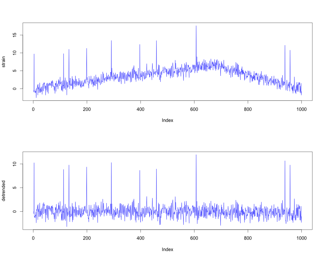
If I simulate your signal and apply the DC Blocker to it, the results are in the figure below.

It should preserve the peaks well.

R code to implement it below.

enter image description here

How to choose $\alpha$ ?

This really depends on what you are going to use the data for later. If it's a control application, then phase is probably important to you.

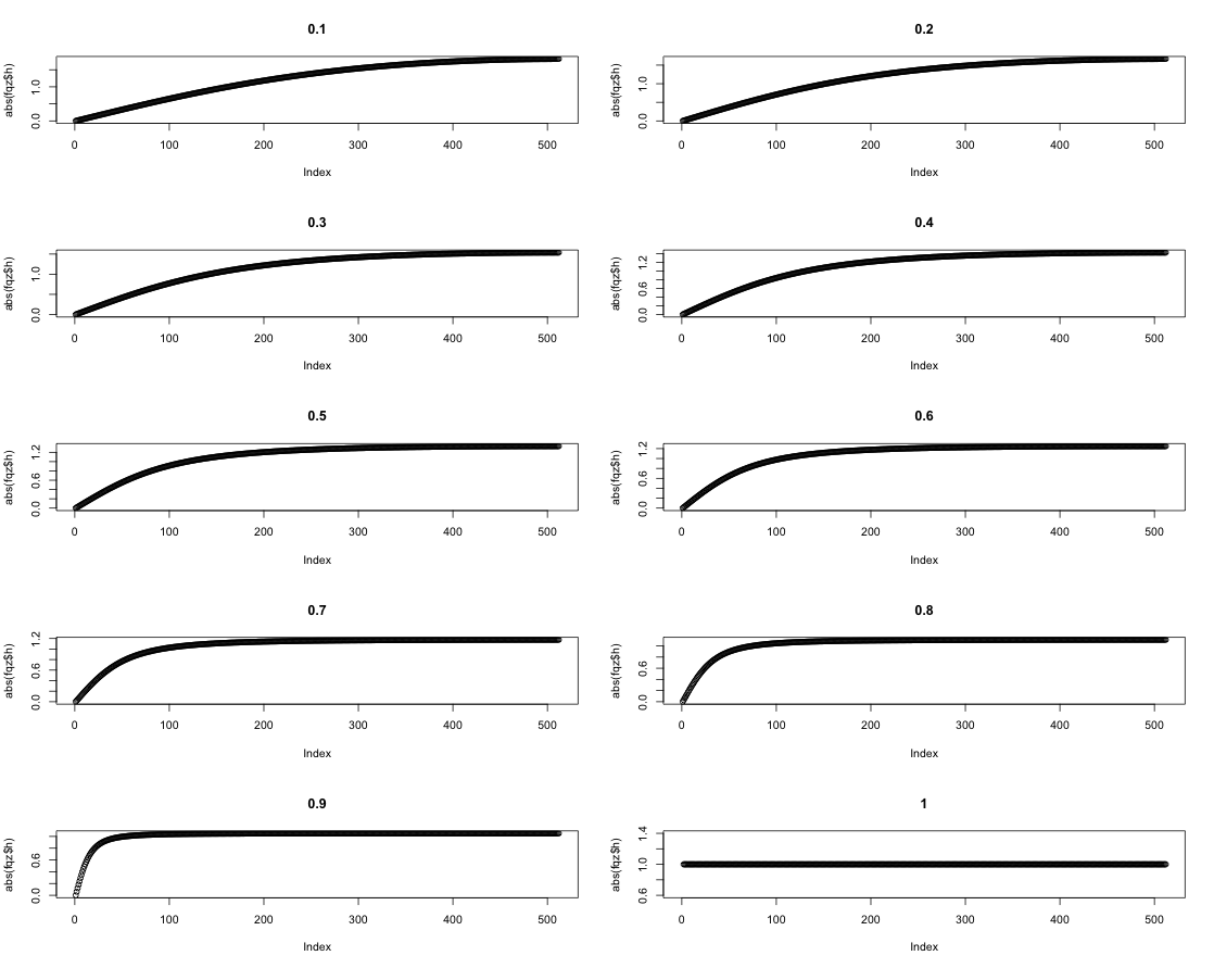
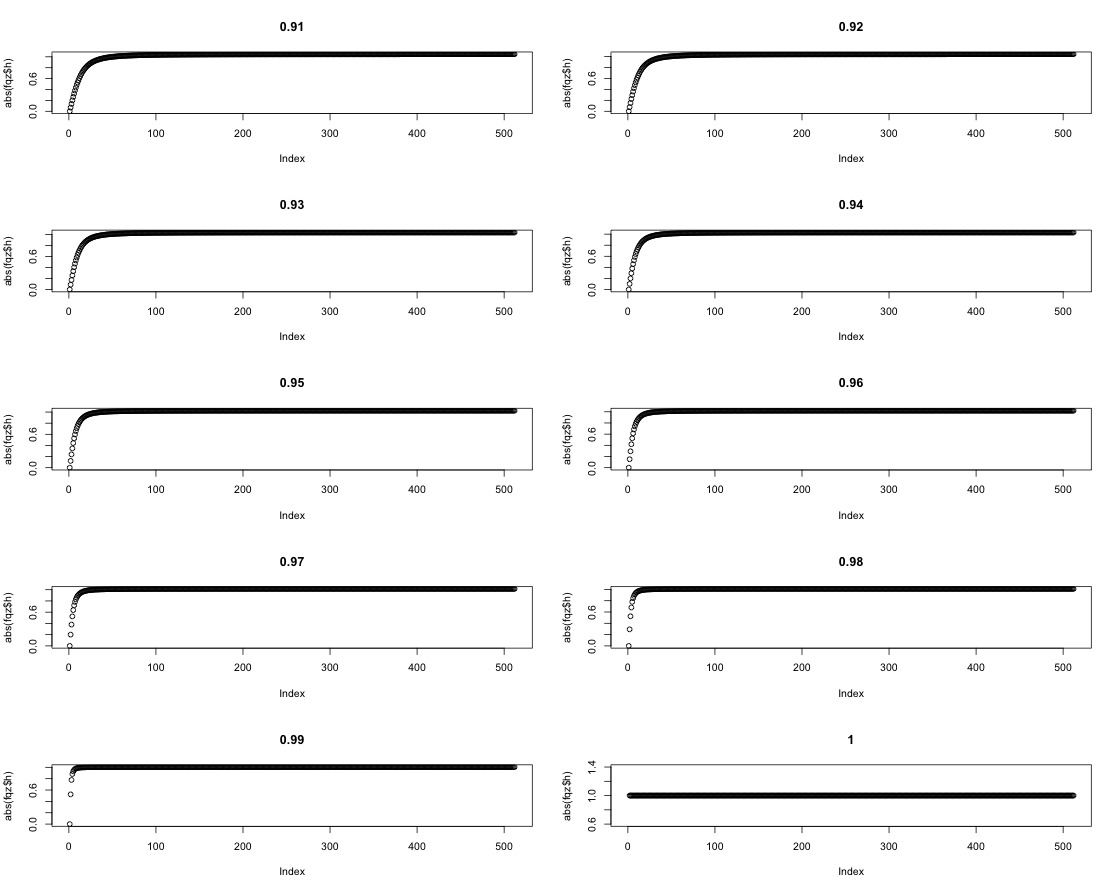
More generally, you want to JUST remove the DC component and not much else. In that case, just look at the magnitude frequency response of the filter.

As you can see from the plots below, low values of $\alpha$ (less than $0.9$ tend to have a bigger impact on the lower frequencies. Hence, I tend to use values of $\alpha$ between $0.9$ and $1.0$.

enter image description here

enter image description here


R Code Below

#27468

T <- 1000
Npeaks <- 10

idx_peaks <- runif(Npeaks,1,T)

strain <- rnorm(T) + c(seq(1,2*T/3,1) ,seq(2*T/3+1,0,-2))/100

strain[idx_peaks] <- strain[idx_peaks] + 10

detrended <- 0*strain
alpha <- 0.9

for (k in 1:length(strain))
{
  if (k>1)
  {
    detrended[k] <- alpha*detrended[k-1] + strain[k] - strain[k-1]
  }
  else
  {
    detrended[k] <- 0
  }
}

par(mfrow=c(2,1))
plot(strain,col="blue", type="l")
plot(detrended,col="blue", type="l")

The usual first approach to this is to use a DC Blocker: $$ y[n] = \alpha*y[n-1] + x[n] - x[n-1] $$ where $0 < \alpha < 1$, $y$ is the DC blocked signal and $x$ is your original signal.

If I simulate your signal and apply the DC Blocker to it, the results are in the figure below.

It should preserve the peaks well.

R code to implement it below.

enter image description here

How to choose $\alpha$ ?

This really depends on what you are going to use the data for later. If it's a control application, then phase is probably important to you.

More generally, you want to JUST remove the DC component and not much else. In that case, just look at the magnitude frequency response of the filter.

As you can see from the plots below, low values of $\alpha$ (less than $0.9$ tend to have a bigger impact on the lower frequencies. Hence, I tend to use values of $\alpha$ between $0.9$ and $1.0$.

enter image description here

enter image description here


R Code Below

#27468

T <- 1000
Npeaks <- 10

idx_peaks <- runif(Npeaks,1,T)

strain <- rnorm(T) + c(seq(1,2*T/3,1) ,seq(2*T/3+1,0,-2))/100

strain[idx_peaks] <- strain[idx_peaks] + 10

detrended <- 0*strain
alpha <- 0.9

for (k in 1:length(strain))
{
  if (k>1)
  {
    detrended[k] <- alpha*detrended[k-1] + strain[k] - strain[k-1]
  }
  else
  {
    detrended[k] <- 0
  }
}

par(mfrow=c(2,1))
plot(strain,col="blue", type="l")
plot(detrended,col="blue", type="l")
The usual first approach to this is to use a DC Blocker: $$ y[n] = \alpha y[n-1] + x[n] - x[n-1] $$ where $0 < \alpha < 1$, $y$ is the DC blocked signal and $x$ is your original signal.

If I simulate your signal and apply the DC Blocker to it, the results are in the figure below.

It should preserve the peaks well.

R code to implement it below.

enter image description here

How to choose $\alpha$ ?

This really depends on what you are going to use the data for later. If it's a control application, then phase is probably important to you.

More generally, you want to JUST remove the DC component and not much else. In that case, just look at the magnitude frequency response of the filter.

As you can see from the plots below, low values of $\alpha$ (less than $0.9$ tend to have a bigger impact on the lower frequencies. Hence, I tend to use values of $\alpha$ between $0.9$ and $1.0$.

enter image description here

enter image description here


R Code Below

#27468

T <- 1000
Npeaks <- 10

idx_peaks <- runif(Npeaks,1,T)

strain <- rnorm(T) + c(seq(1,2*T/3,1) ,seq(2*T/3+1,0,-2))/100

strain[idx_peaks] <- strain[idx_peaks] + 10

detrended <- 0*strain
alpha <- 0.9

for (k in 1:length(strain))
{
  if (k>1)
  {
    detrended[k] <- alpha*detrended[k-1] + strain[k] - strain[k-1]
  }
  else
  {
    detrended[k] <- 0
  }
}

par(mfrow=c(2,1))
plot(strain,col="blue", type="l")
plot(detrended,col="blue", type="l")
Added alpha choice stuff
Source Link
Peter K.
  • 26k
  • 9
  • 47
  • 93

The usual first approach to this is to use a DC Blocker: $$ y[n] = \alpha*y[n-1] + x[n] - x[n-1] $$ where $0 < \alpha < 1$, $y$ is the DC blocked signal and $x$ is your original signal.

If I simulate your signal and apply the DC Blocker to it, the results are in the figure below.

It should preserve the peaks well.

R code to implement it below.

enter image description here

How to choose $\alpha$ ?

This really depends on what you are going to use the data for later. If it's a control application, then phase is probably important to you.

More generally, you want to JUST remove the DC component and not much else. In that case, just look at the magnitude frequency response of the filter.

As you can see from the plots below, low values of $\alpha$ (less than $0.9$ tend to have a bigger impact on the lower frequencies. Hence, I tend to use values of $\alpha$ between $0.9$ and $1.0$.

enter image description here

enter image description here


R Code Below

#27468

T <- 1000
Npeaks <- 10

idx_peaks <- runif(Npeaks,1,T)

strain <- rnorm(T) + c(seq(1,2*T/3,1) ,seq(2*T/3+1,0,-2))/100

strain[idx_peaks] <- strain[idx_peaks] + 10

detrended <- 0*strain
alpha <- 0.9

for (k in 1:length(strain))
{
  if (k>1)
  {
    detrended[k] <- alpha*detrended[k-1] + strain[k] - strain[k-1]
  }
  else
  {
    detrended[k] <- 0
  }
}

par(mfrow=c(2,1))
plot(strain,col="blue", type="l")
plot(detrended,col="blue", type="l")
The usual first approach to this is to use a DC Blocker: $$ y[n] = \alpha*y[n-1] + x[n] - x[n-1] $$ where $0 < \alpha < 1$, $y$ is the DC blocked signal and $x$ is your original signal.

If I simulate your signal and apply the DC Blocker to it, the results are in the figure below.

It should preserve the peaks well.

R code to implement it below.

enter image description here

How to choose $\alpha$ ?

This really depends on what you are going to use the data for later. If it's a control application, then phase is probably important to you.

More generally, you want to JUST remove the DC component and not much else. In that case, just look at the magnitude frequency response of the filter.

As you can see from the plots below, low values of $\alpha$ (less than $0.9$ tend to have a bigger impact on the lower frequencies. Hence, I tend to use values of $\alpha$ between $0.9$ and $1.0$.

enter image description here

enter image description here


R Code Below

#27468

T <- 1000
Npeaks <- 10

idx_peaks <- runif(Npeaks,1,T)

strain <- rnorm(T) + c(seq(1,2*T/3,1) ,seq(2*T/3+1,0,-2))/100

strain[idx_peaks] <- strain[idx_peaks] + 10

detrended <- 0*strain
alpha <- 0.9

for (k in 1:length(strain))
{
  if (k>1)
  {
    detrended[k] <- alpha*detrended[k-1] + strain[k] - strain[k-1]
  }
  else
  {
    detrended[k] <- 0
  }
}

par(mfrow=c(2,1))
plot(strain,col="blue", type="l")
plot(detrended,col="blue", type="l")
Source Link
Peter K.
  • 26k
  • 9
  • 47
  • 93

The usual first approach to this is to use a DC Blocker: $$ y[n] = \alpha*y[n-1] + x[n] - x[n-1] $$ where $0 < \alpha < 1$, $y$ is the DC blocked signal and $x$ is your original signal.

If I simulate your signal and apply the DC Blocker to it, the results are in the figure below.

It should preserve the peaks well.

R code to implement it below.

enter image description here


R Code Below

#27468

T <- 1000
Npeaks <- 10

idx_peaks <- runif(Npeaks,1,T)

strain <- rnorm(T) + c(seq(1,2*T/3,1) ,seq(2*T/3+1,0,-2))/100

strain[idx_peaks] <- strain[idx_peaks] + 10

detrended <- 0*strain
alpha <- 0.9

for (k in 1:length(strain))
{
  if (k>1)
  {
    detrended[k] <- alpha*detrended[k-1] + strain[k] - strain[k-1]
  }
  else
  {
    detrended[k] <- 0
  }
}

par(mfrow=c(2,1))
plot(strain,col="blue", type="l")
plot(detrended,col="blue", type="l")