Corrected language
Source Link
jojeck
  • 11.2k
  • 6
  • 38
  • 75

I think you should plot something like:

t = [0:0.05:1];      %20Hz sampling
a = sin(2*pi*2*t);   %2Hz sine wave
b = sin(2*pi*18*t);  %18Hz sine wave
plot(t, a, 'bo');
hold on;
plot(t, b, 'ro');

T = [0:0.001:1];     %1000Hz sampling frequency
A = sin(2*pi*2*T);
B = sin(2*pi*18*T);
% plot for 1000Hz sampling frequency
plot(T, A, 'b');
plot(T, B, 'r');

legend({'2Hz @ 20 Hz f_s', '18Hz @ 20 Hz f_s', '2Hz @ 1000 Hz f_s', '18Hz @ 1000 Hz f_s'})

Giving understandingThat allows to understand which exact samples of your sinusoids you are takingtaken at a given sampling frequency:
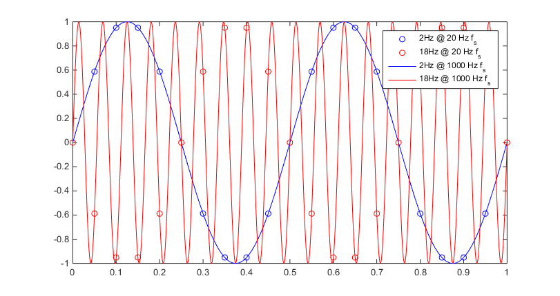
enter image description here

I think you should plot something like:

t = [0:0.05:1];      %20Hz sampling
a = sin(2*pi*2*t);   %2Hz sine wave
b = sin(2*pi*18*t);  %18Hz sine wave
plot(t, a, 'bo');
hold on;
plot(t, b, 'ro');

T = [0:0.001:1];     %1000Hz sampling frequency
A = sin(2*pi*2*T);
B = sin(2*pi*18*T);
% plot for 1000Hz sampling frequency
plot(T, A, 'b');
plot(T, B, 'r');

legend({'2Hz @ 20 Hz f_s', '18Hz @ 20 Hz f_s', '2Hz @ 1000 Hz f_s', '18Hz @ 1000 Hz f_s'})

Giving understanding which exact samples of your sinusoids you are taking at a given sampling frequency:

enter image description here

I think you should plot something like:

t = [0:0.05:1];      %20Hz sampling
a = sin(2*pi*2*t);   %2Hz sine wave
b = sin(2*pi*18*t);  %18Hz sine wave
plot(t, a, 'bo');
hold on;
plot(t, b, 'ro');

T = [0:0.001:1];     %1000Hz sampling frequency
A = sin(2*pi*2*T);
B = sin(2*pi*18*T);
% plot for 1000Hz sampling frequency
plot(T, A, 'b');
plot(T, B, 'r');

legend({'2Hz @ 20 Hz f_s', '18Hz @ 20 Hz f_s', '2Hz @ 1000 Hz f_s', '18Hz @ 1000 Hz f_s'})

That allows to understand which exact samples of your sinusoids you are taken at a given sampling frequency:

enter image description here

edited body
Source Link
jojeck
  • 11.2k
  • 6
  • 38
  • 75

I think you should plot something like:

t = [0:0.05:1];      %20Hz sampling
a = sin(2*pi*2*t);   %2Hz sine wave
b = sin(2*pi*18*t);  %18Hz sine wave
plot(t, a, 'bo');
hold on;
plot(t, b, 'ro');

T = [0:0.001:1];     %100Hz%1000Hz sampling frequency
A = sin(2*pi*2*T);
B = sin(2*pi*18*T);
% plot for 100Hz1000Hz sampling frequency
plot(T, A, 'b');
plot(T, B, 'r');

legend({'2Hz @ 20 Hz f_s', '18Hz @ 20 Hz f_s', '2Hz @ 1001000 Hz f_s', '18Hz @ 1001000 Hz f_s'})

Giving understanding which exact samples of your sinusoids you are taking at a given sampling frequency:

enter image description hereenter image description here

I think you should plot something like:

t = [0:0.05:1];      %20Hz sampling
a = sin(2*pi*2*t);   %2Hz sine wave
b = sin(2*pi*18*t);  %18Hz sine wave
plot(t, a, 'bo');
hold on;
plot(t, b, 'ro');

T = [0:0.001:1];     %100Hz sampling frequency
A = sin(2*pi*2*T);
B = sin(2*pi*18*T);
% plot for 100Hz sampling frequency
plot(T, A, 'b');
plot(T, B, 'r');

legend({'2Hz @ 20 Hz f_s', '18Hz @ 20 Hz f_s', '2Hz @ 100 Hz f_s', '18Hz @ 100 Hz f_s'})

Giving understanding which exact samples of your sinusoids you are taking at a given sampling frequency:

enter image description here

I think you should plot something like:

t = [0:0.05:1];      %20Hz sampling
a = sin(2*pi*2*t);   %2Hz sine wave
b = sin(2*pi*18*t);  %18Hz sine wave
plot(t, a, 'bo');
hold on;
plot(t, b, 'ro');

T = [0:0.001:1];     %1000Hz sampling frequency
A = sin(2*pi*2*T);
B = sin(2*pi*18*T);
% plot for 1000Hz sampling frequency
plot(T, A, 'b');
plot(T, B, 'r');

legend({'2Hz @ 20 Hz f_s', '18Hz @ 20 Hz f_s', '2Hz @ 1000 Hz f_s', '18Hz @ 1000 Hz f_s'})

Giving understanding which exact samples of your sinusoids you are taking at a given sampling frequency:

enter image description here

Source Link
jojeck
  • 11.2k
  • 6
  • 38
  • 75

I think you should plot something like:

t = [0:0.05:1];      %20Hz sampling
a = sin(2*pi*2*t);   %2Hz sine wave
b = sin(2*pi*18*t);  %18Hz sine wave
plot(t, a, 'bo');
hold on;
plot(t, b, 'ro');

T = [0:0.001:1];     %100Hz sampling frequency
A = sin(2*pi*2*T);
B = sin(2*pi*18*T);
% plot for 100Hz sampling frequency
plot(T, A, 'b');
plot(T, B, 'r');

legend({'2Hz @ 20 Hz f_s', '18Hz @ 20 Hz f_s', '2Hz @ 100 Hz f_s', '18Hz @ 100 Hz f_s'})

Giving understanding which exact samples of your sinusoids you are taking at a given sampling frequency:

enter image description here